5 Reproducible Research Techniques - Data Training
5.1 Writing Good Data Management Plans
5.1.1 Learning Objectives
In this lesson, you will learn:
- Why create data management plans
- The major components of data management plans
- Tools that can help create a data management plan
- Features and functionality of the DMPTool
5.1.2 When to Plan: The Data Life Cycle
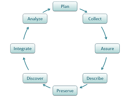
Shown below is one version of the Data Life Cycle that was developed by DataONE. The data life cycle provides a high level overview of the stages involved in successful management and preservation of data for use and reuse. Multiple versions of a data life cycle exist with differences attributable to variation in practices across domains or communities. It is not neccesary for researchers to move through the data life cycle in a cylical fashion and some research activities might use only part of the life cycle. For instance, a project involving meta-analysis might focus on the Discover, Integrate, and Analyze steps, while a project focused on primary data collection and analysis might bypass the Discover and Integrate steps. However, ‘Plan’ is at the top of the data life cycle as it is advisable to initiate your data management planning at the beginning of your research process, before any data has been collected.
5.1.3 Why Plan?
Planning data management in advance povides a number of benefits to the researcher.
- Saves time and increases efficiency; Data management planning requires that a researcher think about data handling in advance of data collection, potentially raising any challenges before they are encountered.
- Engages your team; Being able to plan effectively will require conversation with multiple parties, engaging project participants from the outset.
- Allows you to stay organized; It will be easier to organize your data for analysis and reuse.
- Meet funder requirements; Funders require a data management plan as part of the proposal process.
- Share data; Information in the DMP is the foundation for archiving and sharing data with community.
5.1.4 How to Plan
- As indicated above, engaging your team is a benefit of data management planning. Collaborators involved in the data collection and processing of your research data bring diverse expertise. Therefore, plan in collaboration with these individuals.
- Make sure to plan from the start to avoid confusion, data loss, and increase efficiency. Given DMPs are a requirement of funding agencies, it is nearly always neccesary to plan from the start. However, the same should apply to research that is being undertaken outside of a specific funded proposal.
- Make sure to utilize resources that are available to assist you in helping to write a good DMP. These might include your institutional library or organization data manager, online resources or education materials such as these.
- Use tools available to you; you don’t have to reinvent the wheel.
- Revise your plan as situations change and you potentially adapt/alter your project. Like your research projects, data management plans are not static, they require changes and updates throughout the research project process.
5.1.5 What to include in a DMP
If you are writing a data management plan as part of a solicitation proposal, the funding agency will have guidelines for the information they want to be provided in the plan. A good plan will provide information on the study design; data to be collected; metadata; policies for access, sharing & reuse; long-term storage & data management; and budget.
A note on Metadata: Both basic metadata (such as title and researcher contact information) and comprehensive metadata (such as complete methods of data collection) are critical for accurate interpretation and understanding. The full definitions of variables, especially units, inside each dataset are also critical as they relate to the methods used for creation. Knowing certain blocking or grouping methods, for example, would be necessary to understand studies for proper comparisons and synthesis.
5.1.6 NSF DMP requirements
In the 2014 Proposal Preparation Instructions, Section J ‘Special Information and Supplementary Documentation’ NSF put foward the baseline requirements for a data management plan. In addition, there are specific divison and program requirements that provide additional detail. If you are working on a research project with funding that does not require a data management plan, or are developing a plan for unfunded research, the NSF generic requirements are a good set of guidelines to follow.
Five Sections of the NSF DMP Requirements
1. Products of research
Types of data, samples, physical collections, software, curriculum materials, other materials produced during project
2. Data formats and standards
Standards to be used for data and metadata format and content (for initial data collection, as well as subsequent storageand processing)
3. Policies for access and sharing
Provisions for appropriate protection of privacy, confidentiality, security, intellectual property, or other rights or requirements
4. Policies and provisions for re-use
Including re-distribution and the production of derivatives
5. Archiving of data
Plans for archiving data, samples, research products and for preservation of access
5.1.7 Tools in Support of Creating a DMP

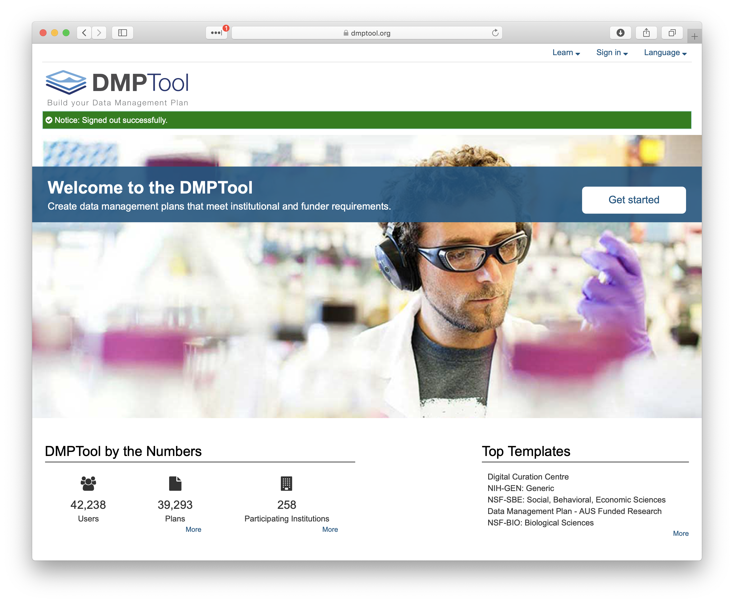
The DMP Tool and DMP Online are both easy to use web based tools that support the development of a DMP. The tools are partnered and share a code base; the DMPTool incorporates templates from US funding agencies and the DMP Online is focussed on EU requirements.
5.1.8 NSF (and other) Template Support for DMPs
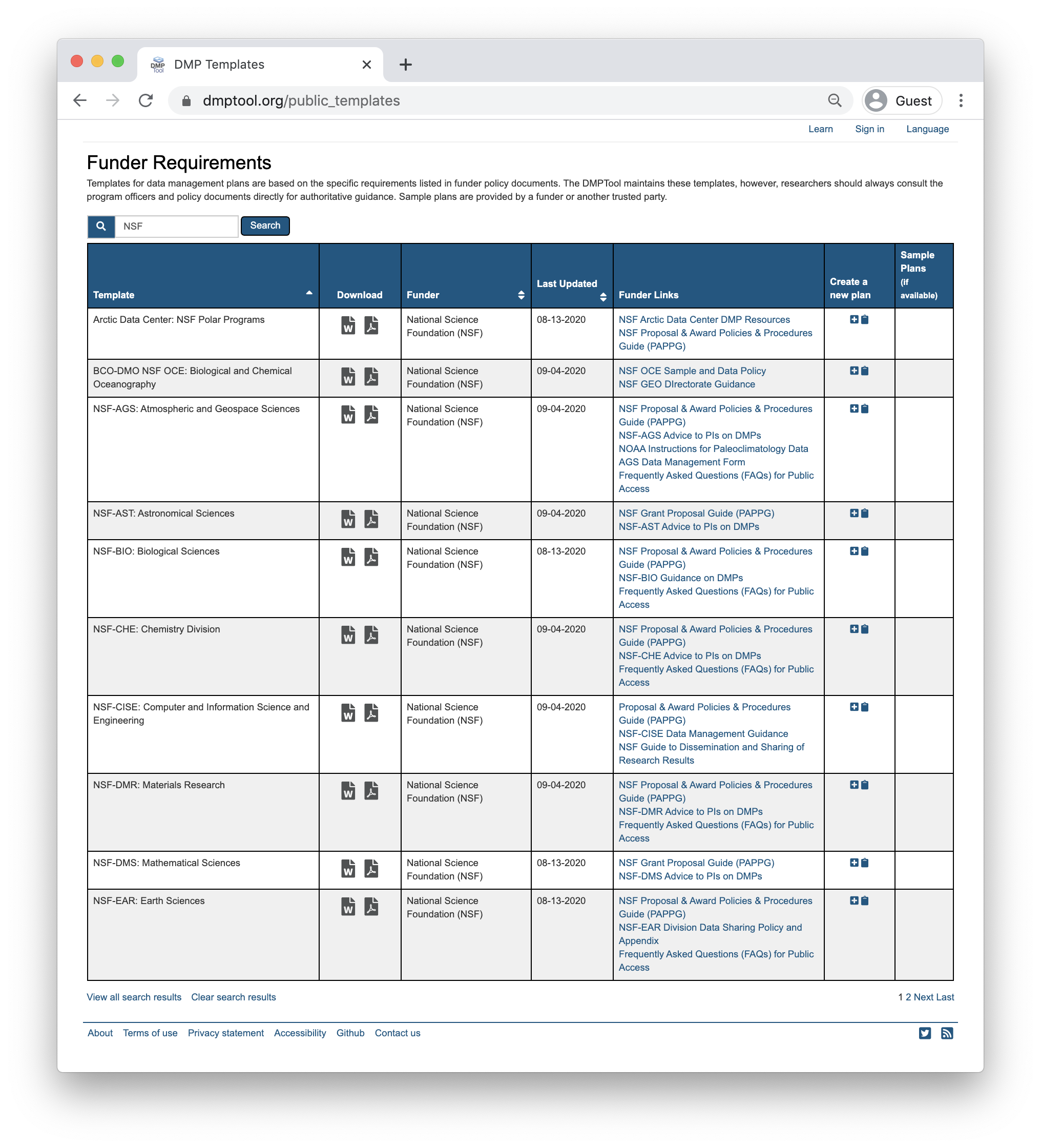
To support researchers in creating Data Management Plans that fulfil funder requirements, the DMPTool includes templates for multiple funders and agencies. These templates form the backbone of the tool structure and enable users to ensure they are responding to specific agency guidelines. There is a template for NSF-BIO, NSF-EAR as well as other NSF Divisions. If your specific agency or division is not represented, the NSF-GEN (generic) template is a good choice to work from.
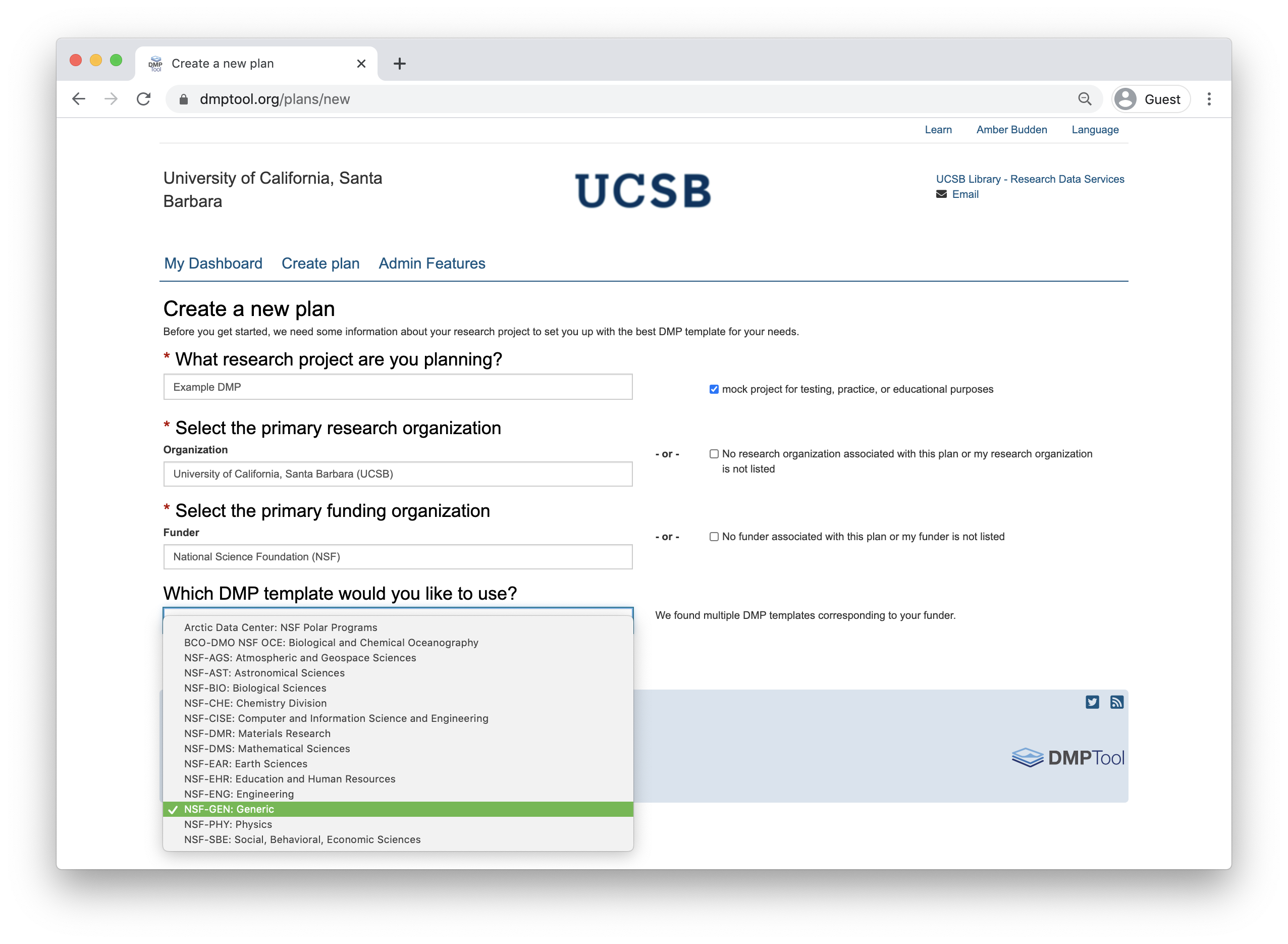
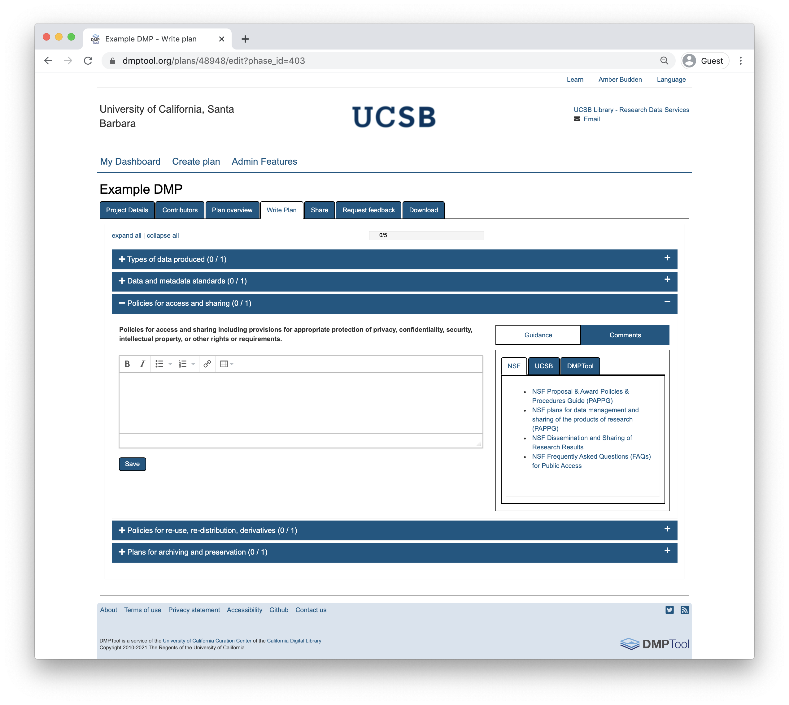
When creating a new plan, indicate that your funding agency is the National Science Foundation and you will then have the option to select a template. Below is the example with NSF-GEN.
As you answer the questions posed, guidance information from the NSF, the DMPTool and your institution (if applicable) will be visible under the ‘Guidance’ tab on the right hand side. In some cases, the template may include an example answer at the bottom. If so, it is not intended that you copy and paste this verbatim. Rather, this is example prose that you can refer to for answering the question.
5.1.10 Additional Resources
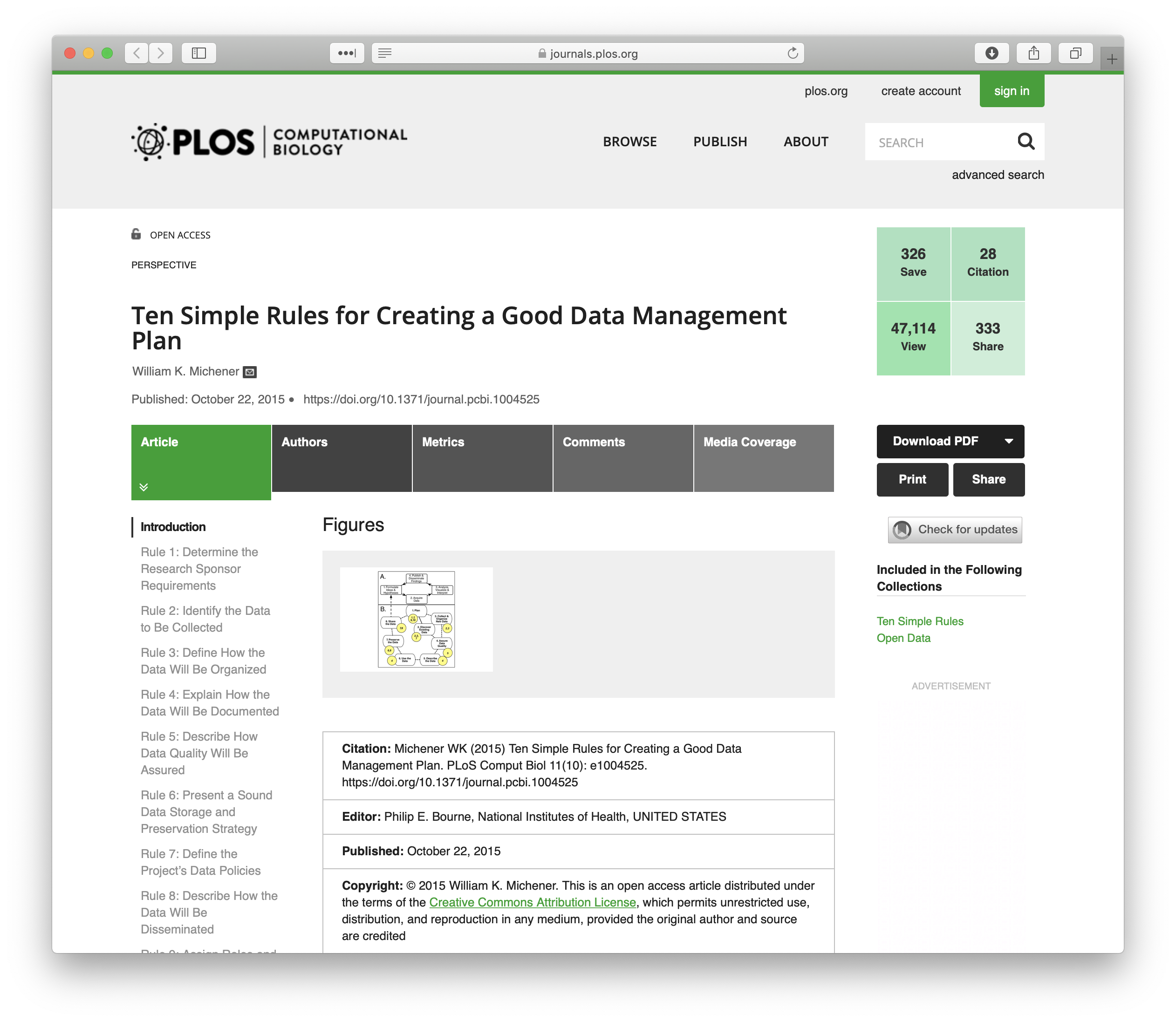
The article Ten Simple Rules for Creating a Good Data Management Plan is a great resource for thinking about writing a data management plan and the information you should include within the plan.
5.2 Reproducible Research, RStudio and Git/GitHub Setup
5.2.1 Learning Objectives
In this lesson, you will learn:
- Why reproducibility in research is useful
- What is meant by computational reproducibility
- How to check to make sure your RStudio environment is set up properly for analysis
- How to set up git
5.2.2 Introduction to reproducible research
Reproducibility is the hallmark of science, which is based on empirical observations coupled with explanatory models. And reproducible research is at the core of what we do at NCEAS, research synthesis.
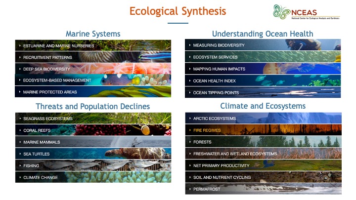
The National Center for Ecological Analysis and Synthesis was funded over 25 years ago to bring together interdisciplinary researchers in exploration of grand challenge ecological questions through analysis of existing data. Such questions often require integration, analysis and synthesis of diverse data across broad temporal, spatial and geographic scales. Data that is not typically collected by a single individual or collaborative team. Synthesis science, leveraging previously collected data, was a novel concept at that time and the approach and success of NCEAS has been a model for other synthesis centers.
 During this course you will learn about some of the challenges that can be encountered when working with published data, but more importantly, how to apply best practices to data collection, documentation, analysis and management to mitigate these challenges in support of reproducible research.
Why is reproducible research important?
Working in a reproducible manner builds efficiencies into your own research practices. The ability to automate processes and rerun analyses as you collect more data, or share your full workflow (including data, code and products) with colleagues, will accelerate the pace of your research and collaborations. However, beyond these direct benefits, reproducible research builds trust in science with the public, policy makers and others.
What data were used in this study? What methods applied? What were the parameter settings? What documentation or code are available to us to evaluate the results? Can we trust these data and methods?
Are the results reproducible?
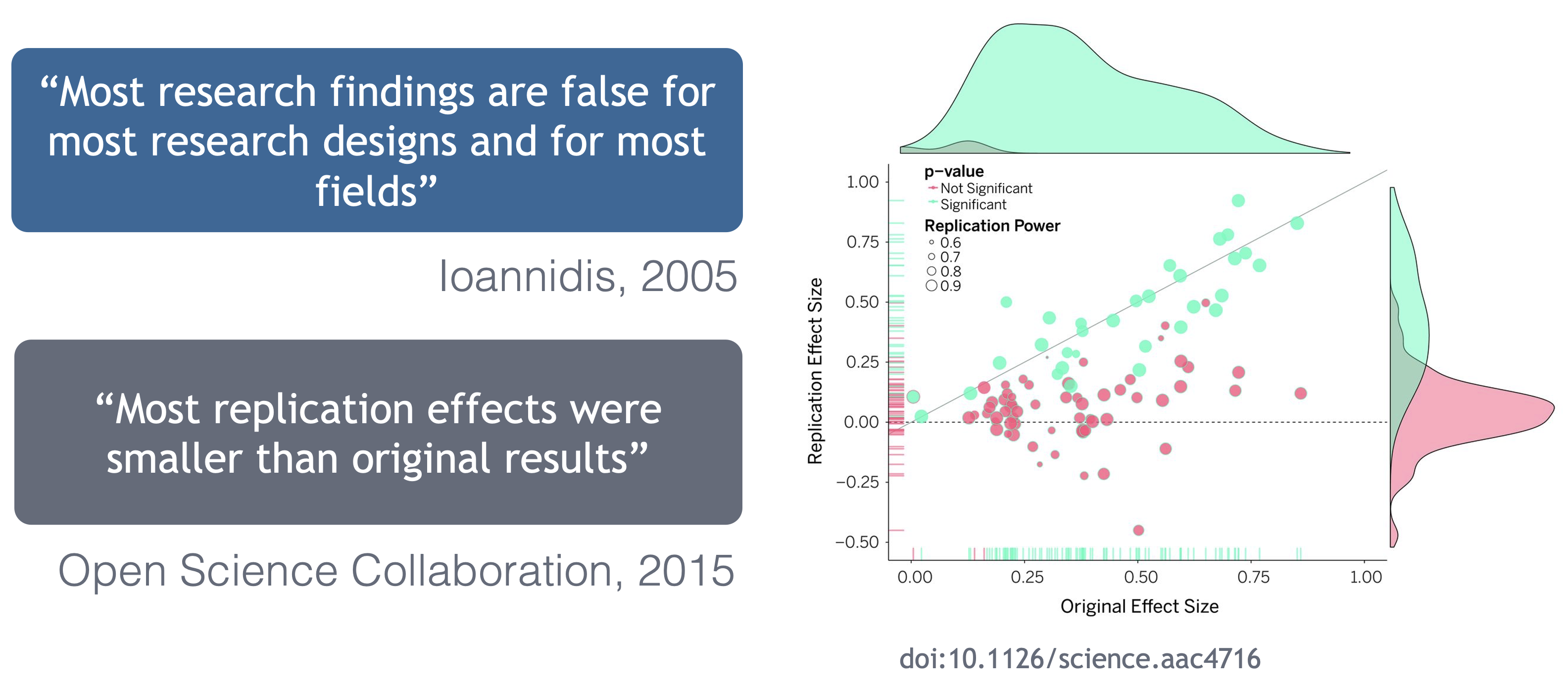
Ionnidis (2005) contends that “Most research findings are false for most research designs and for most fields”, and a study of replicability in psychology experiments found that “Most replication effects were smaller than the original results” (Open Science Collaboration, 2015).
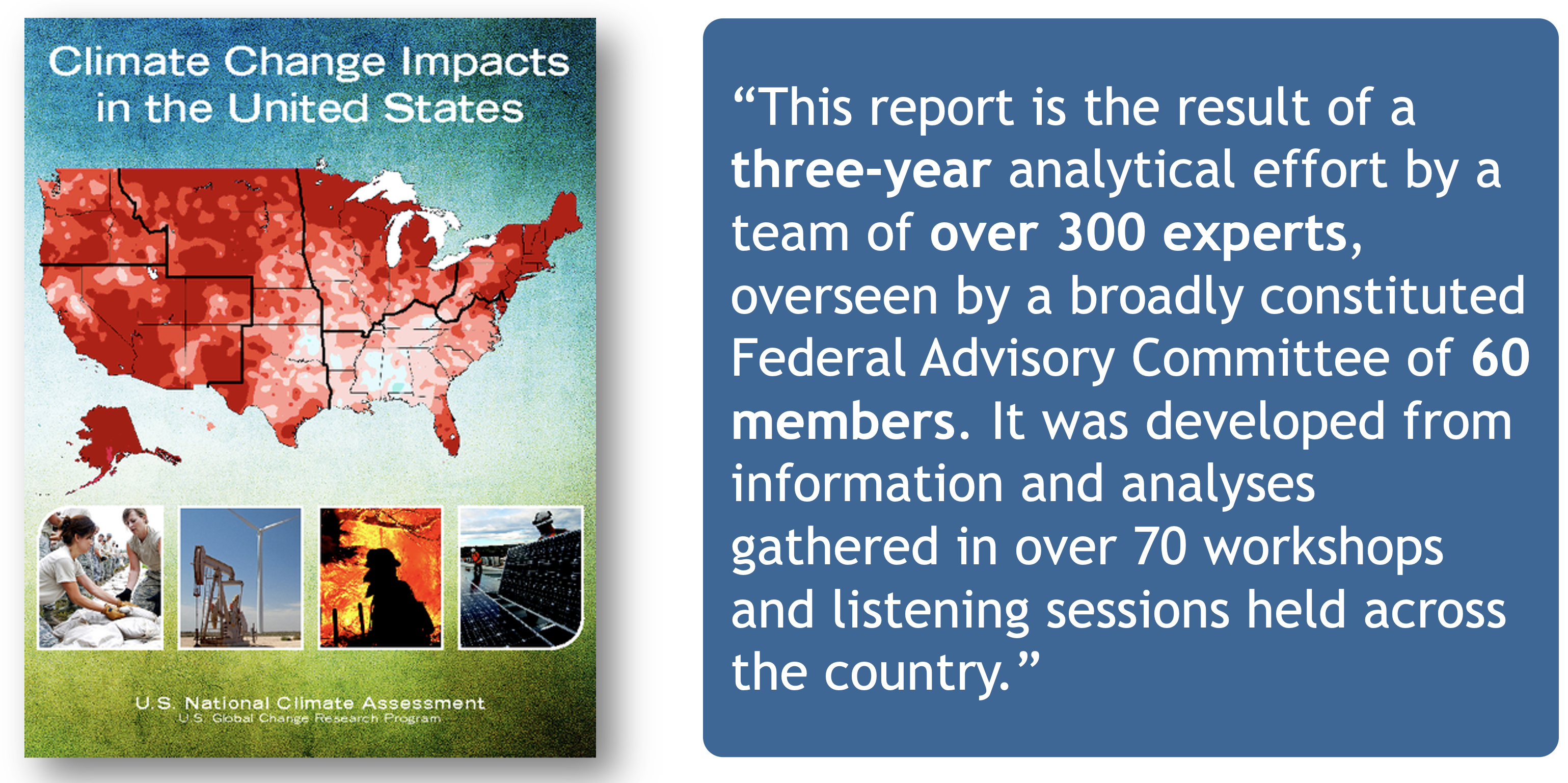
In the case of ‘climategate’, it took three years, and over 300 personnel, to gather the necessary provenance information in order to document how results, figures and other outputs were derived from input sources. Time and effort that could have been significantly reduced with appropriate documentation and reproducible practices. Moving forward, through reproducible research training, practices, and infrastructure, the need to manually chase this information will be reduced enabling replication studies and great trust in science.
Computational reproducibility
While reproducibility encompasses the full science lifecycle, and includes issues such as methodological consistency and treatment of bias, in this course we will focus on computational reproducibility: the ability to document data, analyses, and models sufficiently for other researchers to be able to understand and ideally re-execute the computations that led to scientific results and conclusions.
The first step towards addressing these issues is to be able to evaluate the data, analyses, and models on which conclusions are drawn. Under current practice, this can be difficult because data are typically unavailable, the method sections of papers do not detail the computational approaches used, and analyses and models are often conducted in graphical programs, or, when scripted analyses are employed, the code is not available.
And yet, this is easily remedied. Researchers can achieve computational reproducibility through open science approaches, including straightforward steps for archiving data and code openly along with the scientific workflows describing the provenance of scientific results (e.g., Hampton et al. (2015), Munafò et al. (2017)).
Conceptualizing workflows
Scientific workflows encapsulate all of the steps from data acquisition, cleaning, transformation, integration, analysis, and visualization.
Workflows can range in detail from simple flowcharts to fully executable scripts. R scripts and python scripts are a textual form of a workflow, and when researchers publish specific versions of the scripts and data used in an analysis, it becomes far easier to repeat their computations and understand the provenance of their conclusions.
5.2.2.1 Summary
Computational reproducibility provides:
- transparency by capturing and communicating scientific workflows
- research to stand on the shoulders of giants (build on work that came before)
- credit for secondary usage and supports easy attribution
- increased trust in science
Preserving computational workflows enables understanding, evaluation, and reuse for the benefit of future you and your collaborators and colleagues across disciplines.
Reproducibility means different things to different researchers. For our purposes, practical reproducibility looks like:
- Preserving the data
- Preserving the software workflow
- Documenting what you did
- Describing how to interpret it all
During this course will outline best practices for how to make those four components happen.
5.2.3 Setting up the R environment on your local computer
To get started on the rest of this course, you will need to set up your own computer with the following software so that you can step through the exercises and are ready to take the tools you learn in the course into your daily work.
R Version
We will use R version 4.0.2, which you can download and install from CRAN. To check your version, run this in your RStudio console:
If you have R version 4.0.0 that will likely work fine as well.
RStudio Version
We will be using RStudio version 1.3.1000 or later, which you can download and install here To check your RStudio version, run the following in your RStudio console:
If the output of this does not say 1.2.500 or higher, you should update your RStudio. Do this by selecting Help -> Check for Updates and follow the prompts.
Package installation
Run the following lines to check that all of the packages we need for the training are installed on your computer.
packages <- c("dplyr", "tidyr", "readr", "devtools", "usethis", "roxygen2", "leaflet", "ggplot2", "DT", "scales", "shiny", "sf", "ggmap", "broom", "captioner", "MASS")

for (package in packages) { if (!(package %in% installed.packages())) { install.packages(package) } }
rm(packages) #remove variable from workspace

# Now upgrade any out-of-date packages
update.packages(ask=FALSE)
If you haven’t installed all of the packages, this will automatically start installing them. If they are installed, it won’t do anything.
Next, create a new R Markdown (File -> New File -> R Markdown). If you have never made an R Markdown document before, a dialog box will pop up asking if you wish to install the required packages. Click yes.
At this point, RStudio and R should be all set up.
Setting up git
If you haven’t already, go to github.com and create an account.
Before using git, you need to tell it who you are, also known as setting the global options. The only way to do this is through the command line. Newer versions of RStudio have a nice feature where you can open a terminal window in your RStudio session. Do this by selecting Tools -> Terminal -> New Terminal.
A terminal tab should now be open where your console usually is.
To see if you aleady have your name and email options set, use this command from the terminal:
To set the global options, type the following into the command prompt, with your actual name, and press enter:
Next, enter the following line, with the email address you used when you created your account on github.com:
Note that these lines need to be run one at a time.
Finally, check to make sure everything looks correct by entering these commands, which will return the options that you have set.
Setting up git locally
Every time you set up git on a new computer, the steps we took above to set up git are required. See the above section on setting up git to set your git username and email address.
Note for Windows Users
If you get “command not found” (or similar) when you try these steps through the RStudio terminal tab, you may need to set the type of terminal that gets launched by RStudio. Under some git install scenarios, the git executable may not be available to the default terminal type. Follow the instructions on the RStudio site for Windows specific terminal options. In particular, you should choose “New Terminals open with Git Bash” in the Terminal options (Tools->Global Options->Terminal).
In addition, some versions of windows have difficulty with the command line if you are using an account name with spaces in it (such as “Matt Jones”, rather than something like “mbjones”). You may need to use an account name without spaces.
Updating a previous R installation
This is useful for users who already have R with some packages installed and need to upgrade R, but don’t want to lose packages. If you have never installed R or any R packages before, you can skip this section.
If you already have R installed, but need to update, and don’t want to lose your packages, these two R functions can help you. The first will save all of your packages to a file. The second loads the packages from the file and installs packages that are missing.
Save this script to a file (eg package_update.R).
#' Save R packages to a file. Useful when updating R version
#'
#' @param path path to rda file to save packages to. eg: installed_old.rda
save_packages <- function(path){
    tmp <- installed.packages()
    installedpkgs <- as.vector(tmp[is.na(tmp[,"Priority"]), 1])
    save(installedpkgs, file = path)
}

#' Update packages from a file. Useful when updating R version
#'
#' @param path path to rda file where packages were saved
update_packages <- function(path){
    tmp <- new.env()
    installedpkgs <- load(file = path, envir = tmp)
    installedpkgs <- tmp[[ls(tmp)[1]]]
    tmp <- installed.packages()

    installedpkgs.new <- as.vector(tmp[is.na(tmp[,"Priority"]), 1])
    missing <- setdiff(installedpkgs, installedpkgs.new)
    install.packages(missing)
    update.packages(ask=FALSE)
}
Source the file that you saved above (eg: source(package_update.R)). Then, run the save_packages function.
Then quit R, go to CRAN, and install the latest version of R.
Source the R script that you saved above again (eg: source(package_update.R)), and then run:
This should install all of your R packages that you had before you upgraded.
5.3 Best Practices: Data and Metadata
5.3.1 Learning Objectives
In this lesson, you will learn:
- How to acheive practical reproducibility
- Some best practices for data and metadata management
5.3.2 Best Practices: Overview
The data life cycle has 8 stages: Plan, Collect, Assure, Describe, Preserve, Discover, Integrate, and Analyze. In this section we will cover the following best practices that can help across all stages of the data life cycle:
- Organizing Data
- File Formats
- Large Data Packages
- Metadata
- Data Identifiers
- Provenance
- Licensing and Distribution
5.3.2.1 Organizing Data
We’ll spend an entire lesson later on that’s dedicated to organizing your data in a tidy and effective manner, but first, let’s focus on the benefits on having “clean” data and complete metadata.
- Decreases errors from redundant updates
- Enforces data integrity
- Helps you and future researchers to handle large, complex datasets
- Enables powerful search filtering
Much has been written on effective data management to enable reuse. The following two papers offer words of wisdom:
- Some simple guidelines for effective data management. Borer et al. 2009. Bulletin of the Ecological Society of America.
- Nine simple ways to make it easier to (re)use your data. White et al. 2013. Ideas in Ecology and Evolution 6.
In brief, some of the best practices to follow are:
- Have scripts for all data manipulation that start with the uncorrected raw data file and clean the data programmatically before analysis.
- Design your tables to add rows, not columns. A column should be only one variable and a row should be only one observation.
- Include header lines in your tables
- Use non-proprietary file formats (ie, open source) with descriptive file names without spaces.
Non-proprietary file formats are essential to ensure that your data can still be machine readable long into the future. Open formats include text files and binary formats such as NetCDF.
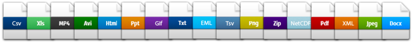
Common switches:
- Microsoft Excel (.xlsx) files - export to text (.txt) or comma separated values (.csv)
- GIS files - export to ESRI shapefiles (.shp)
- MATLAB/IDL - export to NetCDF
When you have or are going to generate large data packages (in the terabytes or larger), it’s important to establish a relationship with the data center early on. The data center can help come up with a strategy to tile data structures by subset, such as by spatial region, by temporal window, or by measured variable. They can also help with choosing an efficient tool to store the data (ie NetCDF or HDF), which is a compact data format that helps parallel read and write libraries of data.
5.3.2.2 Metadata Guidelines
Metadata (data about data) is an important part of the data life cycle because it enables data reuse long after the original collection. Imagine that you’re writing your metadata for a typical researcher (who might even be you!) 30+ years from now - what will they need to understand what’s inside your data files?
The goal is to have enough information for the researcher to understand the data, interpret the data, and then re-use the data in another study.
Another way to think about it is to answer the following questions with the documentation:
- What was measured?
- Who measured it?
- When was it measured?
- Where was it measured?
- How was it measured?
- How is the data structured?
- Why was the data collected?
- Who should get credit for this data (researcher AND funding agency)?
- How can this data be reused (licensing)?
Bibliographic Details
The details that will help your data be cited correctly are:
- a global identifier like a digital object identifier (DOI);
- a descriptive title that includes information about the topic, the geographic location, the dates, and if applicable, the scale of the data
- a descriptive abstract that serves as a brief overview off the specific contents and purpose of the data package
- funding information like the award number and the sponsor;
- the people and organizations like the creator of the dataset (ie who should be cited), the person to contact about the dataset (if different than the creator), and the contributors to the dataset
Discovery Details
The details that will help your data be discovered correctly are:
- the geospatial coverage of the data, including the field and laboratory sampling locations, place names and precise coordinates;
- the temporal coverage of the data, including when the measurements were made and what time period (ie the calendar time or the geologic time) the measurements apply to;
- the taxonomic coverage of the data, including what species were measured and what taxonomy standards and procedures were followed; as well as
- any other contextual information as needed.
Interpretation Details
The details that will help your data be interpreted correctly are:
- the collection methods for both field and laboratory data;
- the full experimental and project design as well as how the data in the dataset fits into the overall project;
- the processing methods for both field and laboratory samples IN FULL;
- all sample quality control procedures;
- the provenance information to support your analysis and modelling methods;
- information about the hardware and software used to process your data, including the make, model, and version; and
- the computing quality control procedures like any testing or code review.
Data Structure and Contents
Well constructed metadata also includes information about the data structure and contents. Everything needs a description: the data model, the data objects (like tables, images, matricies, spatial layers, etc), and the variables all need to be described so that there is no room for misinterpretation.
Variable information includes the definition of a variable, a standardized unit of measurement, definitions of any coded values (such as 0 = not collected), and any missing values (such as 999 = NA).
Not only is this information helpful to you and any other researcher in the future using your data, but it is also helpful to search engines. The semantics of your dataset are crucial to ensure your data is both discoverable by others and interoperable (that is, reusable).
For example, if you were to search for the character string carbon dioxide flux in the general search box at the Arctic Data Center, not all relevant results will be shown due to varying vocabulary conventions (ie, CO2 flux instead of carbon dioxide flux) across disciplines — only datasets containing the exact words carbon dioxide flux are returned. With correct semantic annotation of the variables, your dataset that includes information about carbon dioxide flux but that calls it CO2 flux WOULD be included in that search.
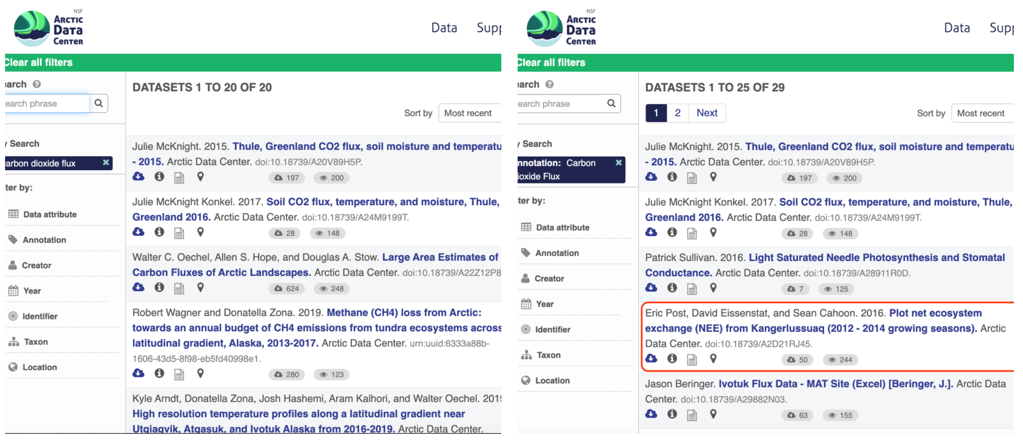
Demonstrates a typical search for “carbon dioxide flux”, yielding 20 datasets. (right) Illustrates an annotated search for “carbon dioxide flux”, yielding 29 datasets. Note that if you were to interact with the site and explore the results of the figure on the right, the dataset in red of Figure 3 will not appear in the typical search for “carbon dioxide flux.”
Rights and Attribution
Correctly assigning a way for your datasets to be cited and reused is the last piece of a complete metadata document. This section sets the scientific rights and expectations for the future on your data, like:
- the citation format to be used when giving credit for the data;
- the attribution expectations for the dataset;
- the reuse rights, which describe who may use the data and for what purpose;
- the redistribution rights, which describe who may copy and redistribute the metadata and the data; and
- the legal terms and conditions like how the data are licensed for reuse.
So, how do you organize all this information? There are a number of metadata standards (think, templates) that you could use, including the Ecological Metadata Language (EML), Geospatial Metadata Standards like ISO 19115 and ISO 19139, the Biological Data Profile (BDP), Dublin Core, Darwin Core, PREMIS, the Metadata Encoding and Transmission Standard (METS), and the list goes on and on. The Arctic Data Center runs on EML.
5.3.3 Data Identifiers
Many journals require a DOI - a digital object identifier - be assigned to the published data before the paper can be accepted for publication. The reason for that is so that the data can easily be found and easily linked to.
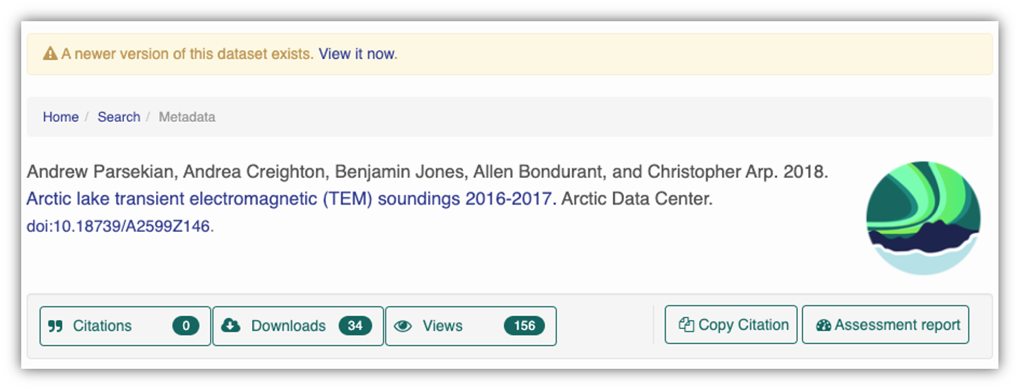
At the Arctic Data Center, we assign a DOI to each published dataset. But, sometimes datasets need to be updated. Each version of a dataset published with the Arctic Data Center has a unique identifier associated with it. Researchers should cite the exact version of the dataset that they used in their analysis, even if there is a newer version of the dataset available. When there is a newer version available, that will be clearly marked on the original dataset page with a yellow banner indicating as such.
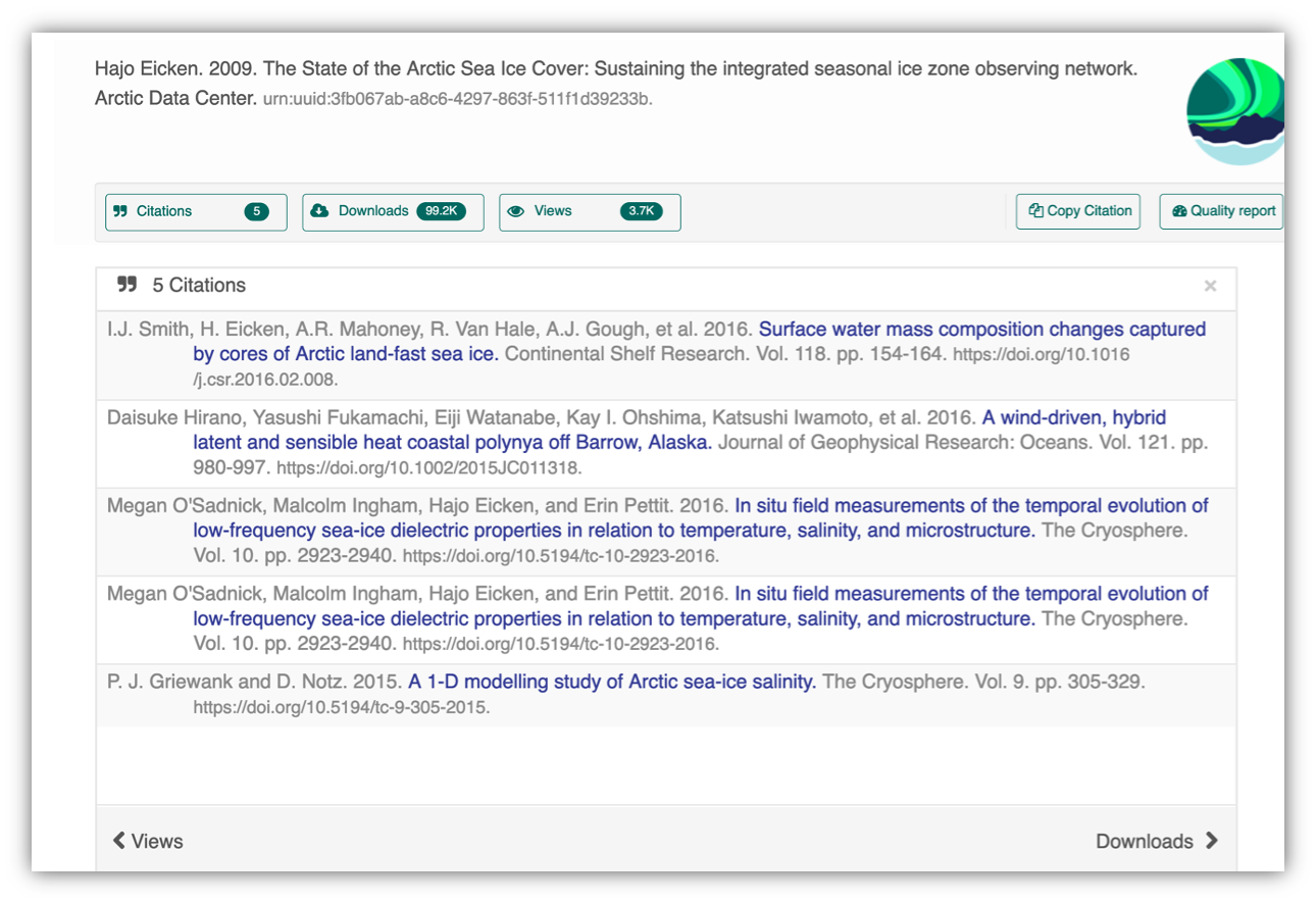
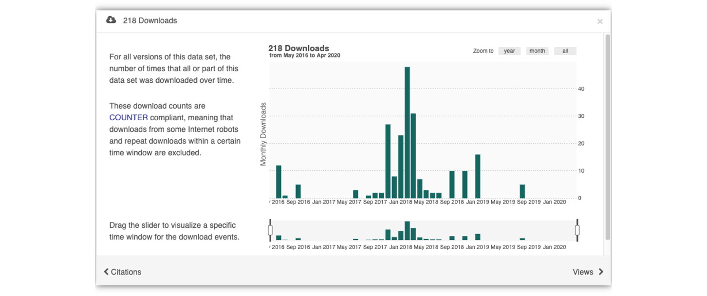
Having the data identified in this manner allows us to accurately track the dataset usage metrics. The Arctic Data Center tracks the number of citations, the number of downloads, and the number of views of each dataset in the catalog.
We filter out most views by internet bots and repeat views within a small time window in order to make these metrics COUNTER compliant. COUNTER is a standard that libraries and repositories use to provide users with consistent, credible, and comparable usage data.
5.3.4 Data Citation
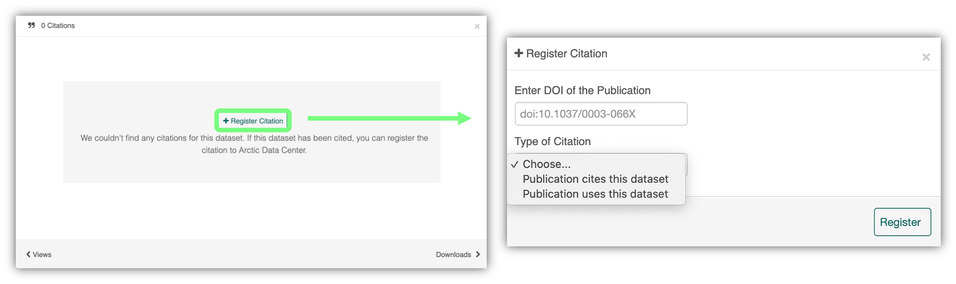
Researchers should get in the habit of citing the data that they use - even if it’s their own data! - in each publication that uses that data. The Arctic Data Center has taken multiple steps towards providing data citation information for all datasets we hold in our catalog, including a feature enabling dataset owners to directly register citations to their datasets.
We recently implemented this “Register Citation” feature to allow researchers to register known citations to their datasets. Researchers may register a citation for any occasions where they know a certain publication uses or refers to a certain dataset, and the citation will be viewable on the dataset profile within 24 hours.
To register a citation, navigate to the dataset using the DOI and click on the citations tab. Once there, this dialog box will pop up and you’ll be able to register the citation with us. Click that button and you’ll see a very simple form asking for the DOI of the paper and if the paper CITES the dataset (that is, the dataset is explicitly identified or linked to somewhere in the text or references) or USES the dataset (that is, uses the dataset but doesn’t formally cite it).
We encourage you to make this part of your workflow, and for you to let your colleagues know about it too!
5.3.5 Provanance & Preserving Computational Workflows
While the Arctic Data Center, Knowledge Network for Biocomplexity, and similar repositories do focus on preserving data, we really set our sights much more broadly on preserving entire computational workflows that are instrumental to advances in science. A computational workflow represents the sequence of computational tasks that are performed from raw data acquisition through data quality control, integration, analysis, modeling, and visualization.
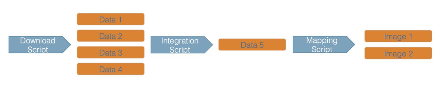
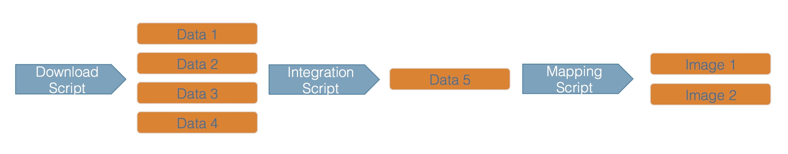
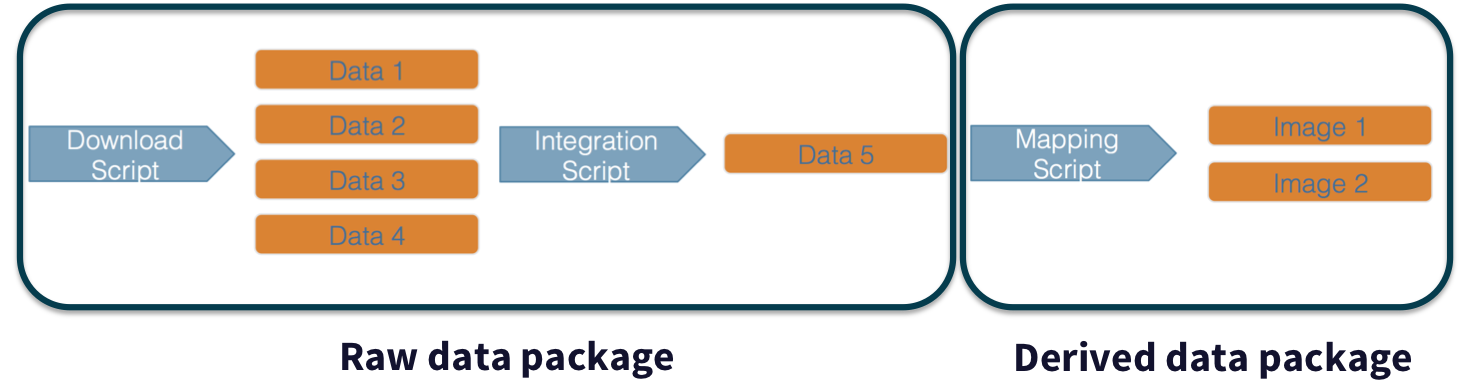
In addition, these workflows are often not executed all at once, but rather are divided into multiple workflows, earch with its own purpose. For example, a data acquistion and cleaning workflow often creates a derived and integrated data product that is then picked up and used by multiple downstream analytical workflows that produce specific scientific findings. These workflows can each be archived as distinct data packages, with the output of the first workflow becoming the input of the second and subsequent workflows.
In an effort to make data more reproducible, datasets also support provenance tracking. With provenance tracking, users of the Arctic Data Center can see exactly what datasets led to what product, using the particular script or workflow that the researcher used.
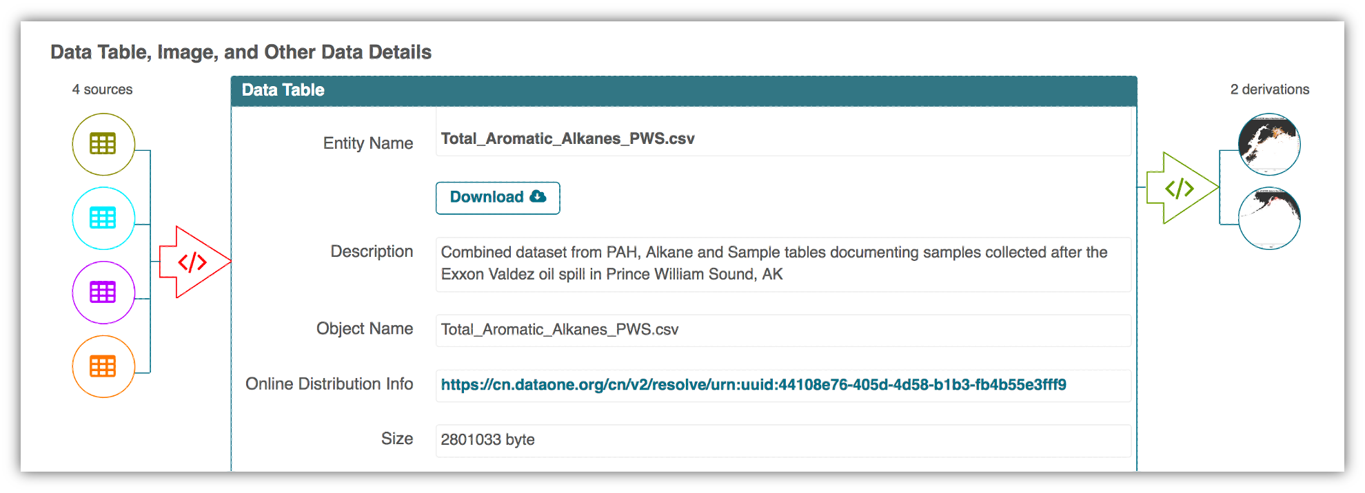
This is a useful tool to make data more compliant with the FAIR principles. In addition to making data more reproducible, it is also useful for building on the work of others; you can produce similar visualizations for another location, for example, using the same code.
RMarkdown itself can be used as a provenance tool, as well - by starting with the raw data and cleaning it programmatically, rather than manually, you preserve the steps that you went through and your workflow is reproducible.

5.4 Data Documentation and Publishing
5.4.1 Learning Objectives
In this lesson, you will learn:
- About open data archives
- What science metadata is and how it can be used
- How data and code can be documented and published in open data archives
5.4.2 Data sharing and preservation
5.4.3 Data repositories: built for data (and code)
- GitHub is not an archival location
- Dedicated data repositories: NEON, KNB, Arctic Data Center, Zenodo, FigShare
- Rich metadata
- Archival in their mission
- Data papers, e.g., Scientific Data
- List of data repositories: http://re3data.org

5.4.4 Metadata
Metadata are documentation describing the content, context, and structure of data to enable future interpretation and reuse of the data. Generally, metadata describe who collected the data, what data were collected, when and where it was collected, and why it was collected.
For consistency, metadata are typically structured following metadata content standards such as the Ecological Metadata Language (EML). For example, here’s an excerpt of the metadata for a sockeye salmon data set:
<?xml version="1.0" encoding="UTF-8"?>
<eml:eml packageId="df35d.442.6" system="knb"
    xmlns:eml="eml://ecoinformatics.org/eml-2.1.1">
    <dataset>
        <title>Improving Preseason Forecasts of Sockeye Salmon Runs through
            Salmon Smolt Monitoring in Kenai River, Alaska: 2005 - 2007</title>
        <creator id="1385594069457">
            <individualName>
                <givenName>Mark</givenName>
                <surName>Willette</surName>
            </individualName>
            <organizationName>Alaska Department of Fish and Game</organizationName>
            <positionName>Fishery Biologist</positionName>
            <address>
                <city>Soldotna</city>
                <administrativeArea>Alaska</administrativeArea>
                <country>USA</country>
            </address>
            <phone phonetype="voice">(907)260-2911</phone>
            <electronicMailAddress>mark.willette@alaska.gov</electronicMailAddress>
        </creator>
        ...
    </dataset>
</eml:eml>
That same metadata document can be converted to HTML format and displayed in a much more readable form on the web: https://knb.ecoinformatics.org/#view/doi:10.5063/F1F18WN4
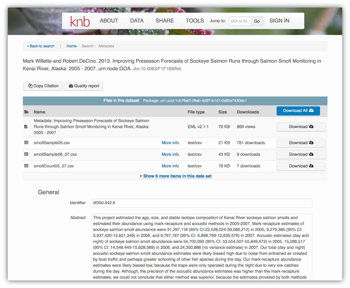 And as you can see, the whole data set or its components can be downloaded and
reused.
And as you can see, the whole data set or its components can be downloaded and
reused.
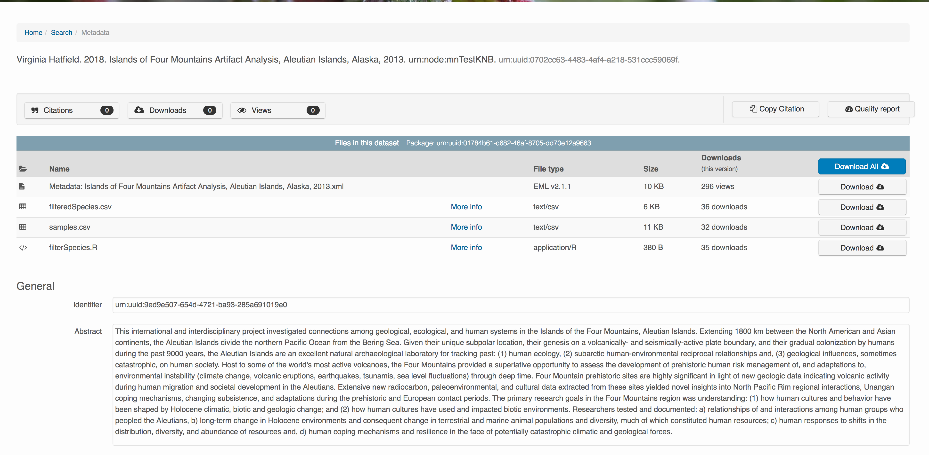
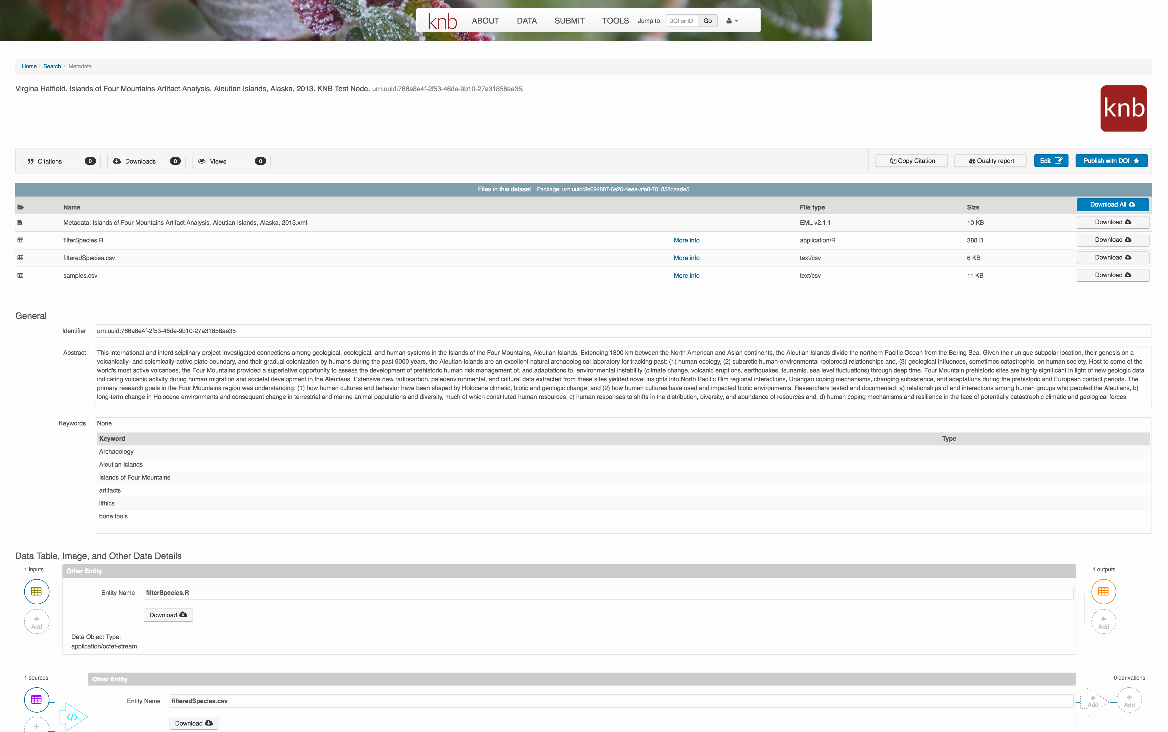
Also note that the repository tracks how many times each file has been downloaded, which gives great feedback to researchers on the activity for their published data.
5.4.5 Structure of a data package
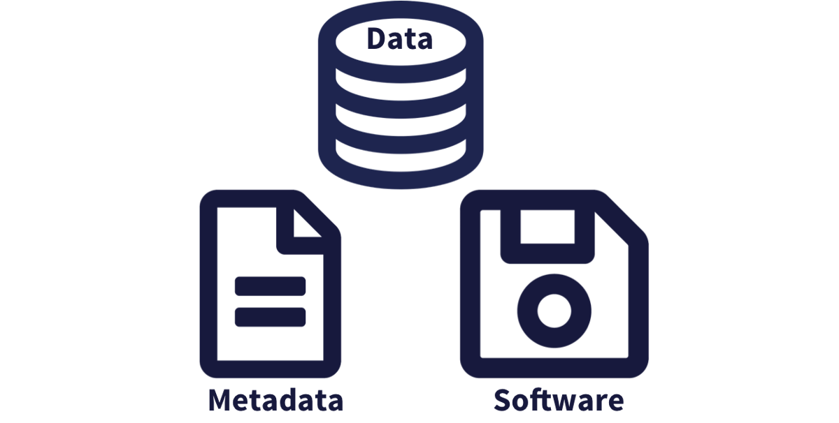
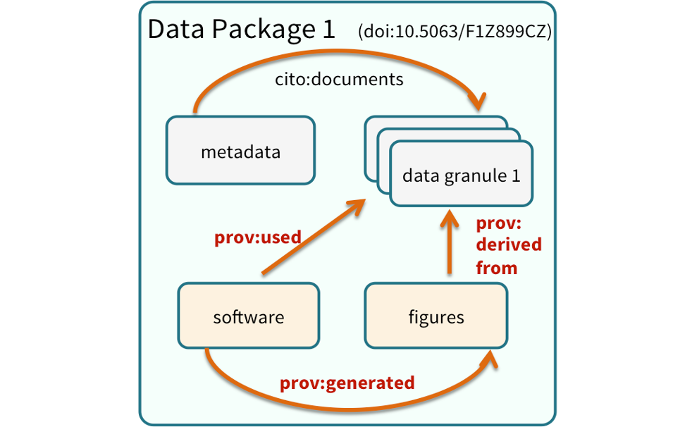
Note that the data set above lists a collection of files that are contained within the data set. We define a data package as a scientifically useful collection of data and metadata that a researcher wants to preserve. Sometimes a data package represents all of the data from a particular experiment, while at other times it might be all of the data from a grant, or on a topic, or associated with a paper. Whatever the extent, we define a data package as having one or more data files, software files, and other scientific products such as graphs and images, all tied together with a descriptive metadata document.
 These data repositories all assign a unique identifier to every version of every
data file, similarly to how it works with source code commits in GitHub. Those identifiers
usually take one of two forms. A DOI identifier is often assigned to the metadata
and becomes the publicly citable identifier for the package. Each of the other files
gets an internal identifier, often a UUID that is globally unique. In the example above,
the package can be cited with the DOI
These data repositories all assign a unique identifier to every version of every
data file, similarly to how it works with source code commits in GitHub. Those identifiers
usually take one of two forms. A DOI identifier is often assigned to the metadata
and becomes the publicly citable identifier for the package. Each of the other files
gets an internal identifier, often a UUID that is globally unique. In the example above,
the package can be cited with the DOI doi:10.5063/F1F18WN4.
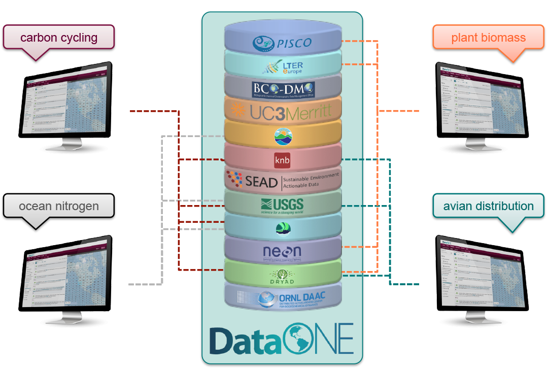
5.4.6 DataONE Federation
DataONE is a federation of dozens of data repositories that work together to make their systems interoperable and to provide a single unified search system that spans the repositories. DataONE aims to make it simpler for researchers to publish data to one of its member repositories, and then to discover and download that data for reuse in synthetic analyses.
DataONE can be searched on the web (https://search.dataone.org/), which effectively allows a single search to find data form the dozens of members of DataONE, rather than visiting each of the currently 43 repositories one at a time.
Publishing data to NEON
Each data repository tends to have its own mechanism for submitting data and providing metadata. At NEON, you will be required to published data to the NEON Data Portal or to an external data repository for specialized data (see externally hosted data).
Full information on data processing, data management and product release can be found in the online NEON Data Management documentation. Below is an overview of the data processing pipeline for observational data.
Web based publishing at the KNB
There’s a broad range of data repositories designed to meet different or specific needs of the researcher community. They may be domain specific, designed to support specialized data, or directly associated with an organization or agency. The Knowledge Network for Biocomplexity is an open data repository hosted by NCEAS that preserves a broad cross section of ecological data. The KNB provides simple web based data package editing and submission forms and the OPTIONAL unit below provides an example of the data submission process for another ecological data repository outside the NEON Data Portal.
Download the data to be used for the tutorial
I’ve already uploaded the test data package, and so you can access the data here:
Grab both CSV files, and the R script, and store them in a convenient folder.
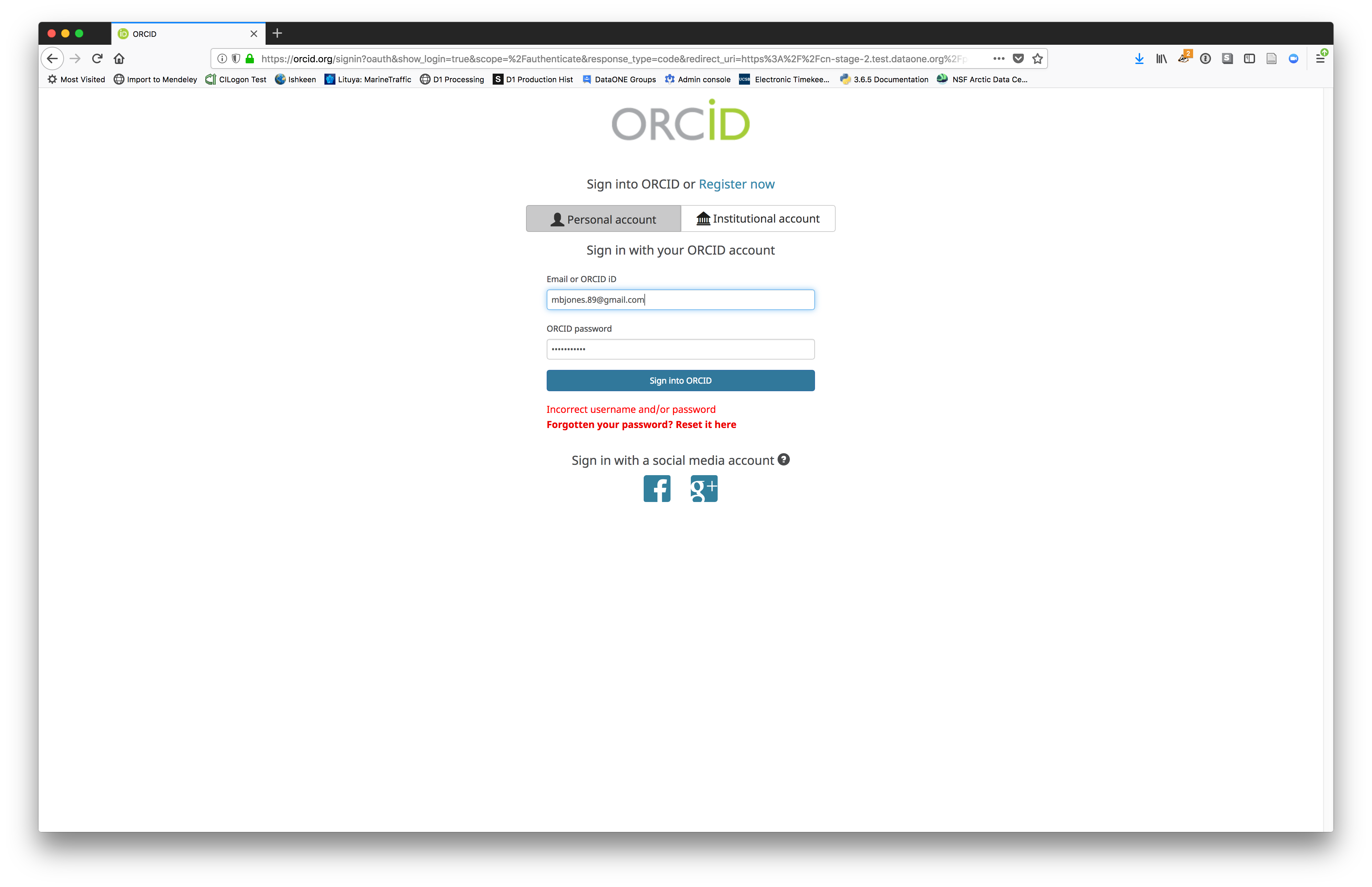
Login via ORCID
We will walk through web submission on https://demo.nceas.ucsb.edu, and start by logging in with an ORCID account. ORCID provides a common account for sharing scholarly data, so if you don’t have one, you can create one when you are redirected to ORCID from the Sign In button.

When you sign in, you will be redirected to orcid.org, where you can either provide your existing ORCID credentials, or create a new account. ORCID provides multiple ways to login, including using your email address, institutional logins from many universities, and logins from social media account providers. Choose the one that is best suited to your use as a scholarly record, such as your university or agency login.
Create and submit the data set
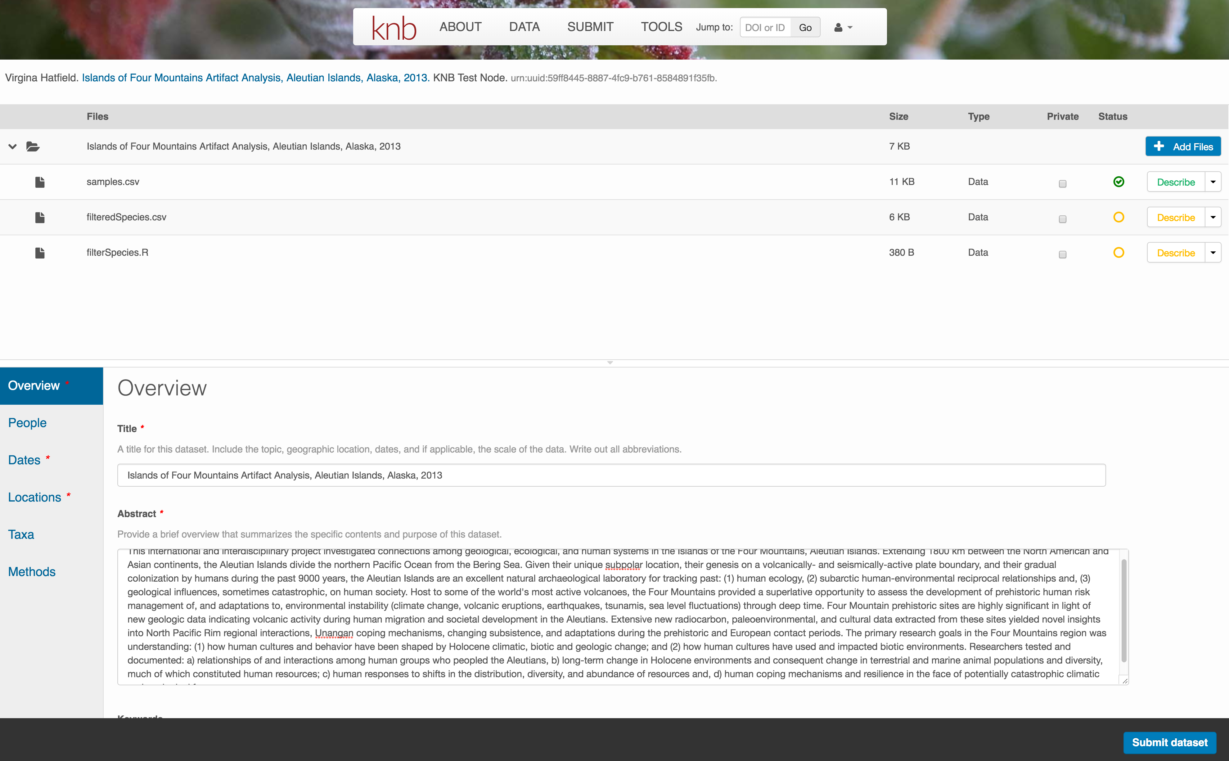
After signing in, you can access the data submission form using the Submit button. Once on the form, upload your data files and follow the prompts to provide the required metadata. Required sections are listed with a red asterisk.
Click Add Files to choose the data files for your package
You can select multiple files at a time to efficiently upload many files.
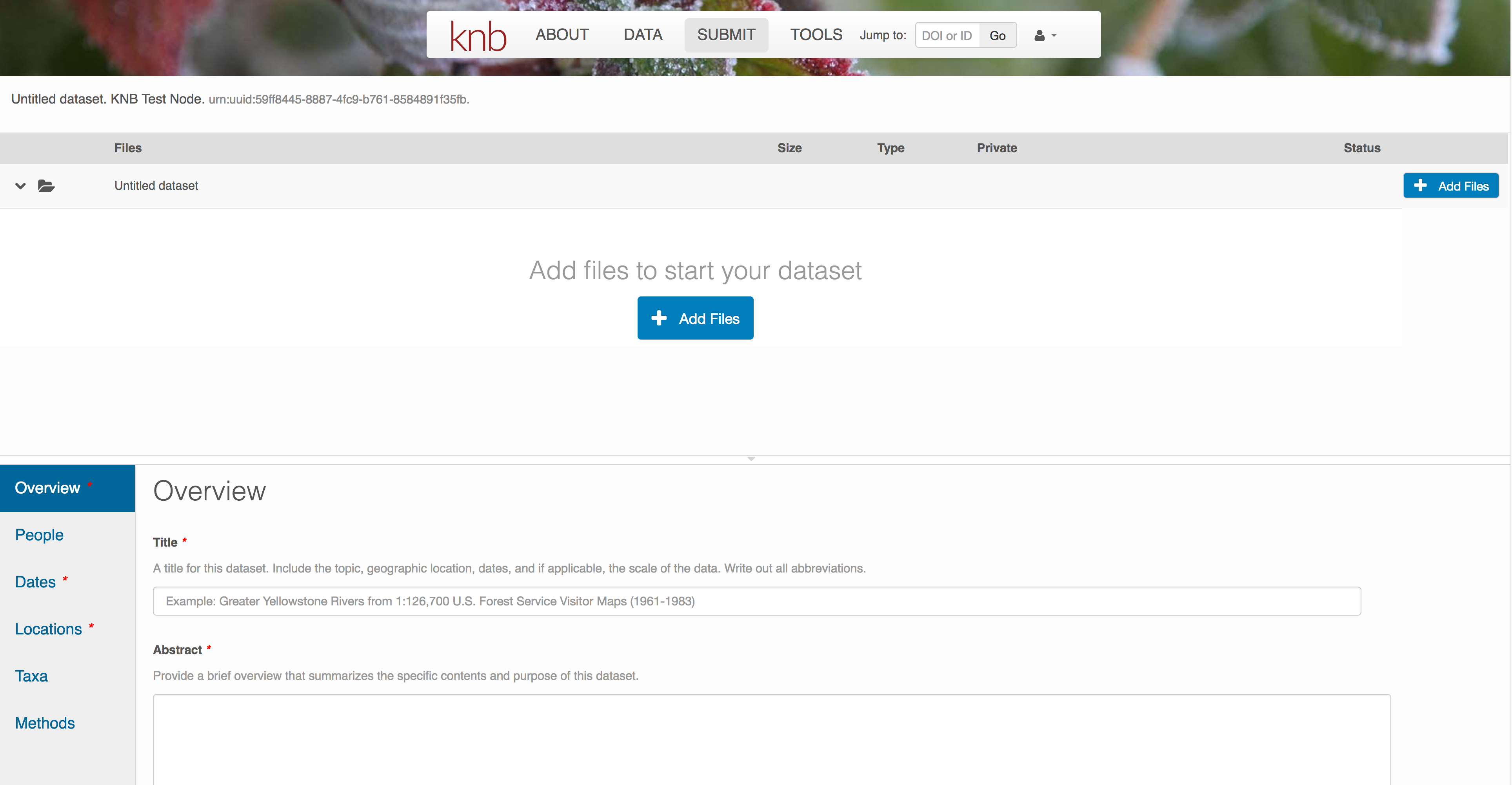
The files will upload showing a progress indicator. You can continue editing metadata while they upload.
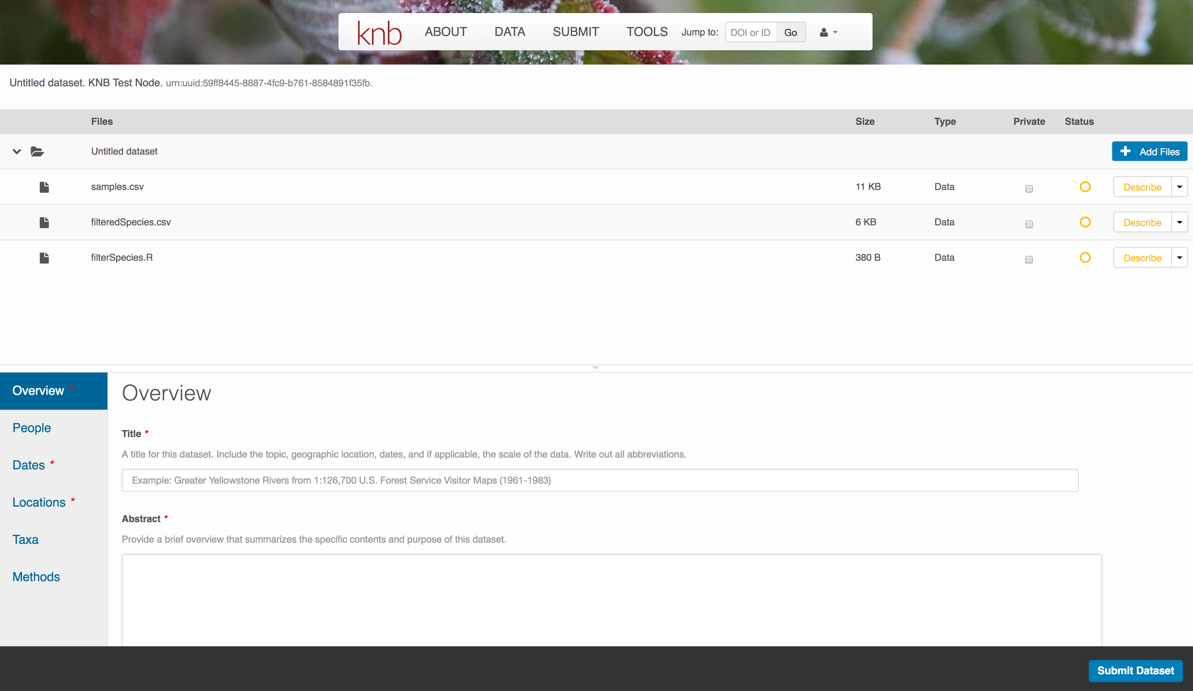
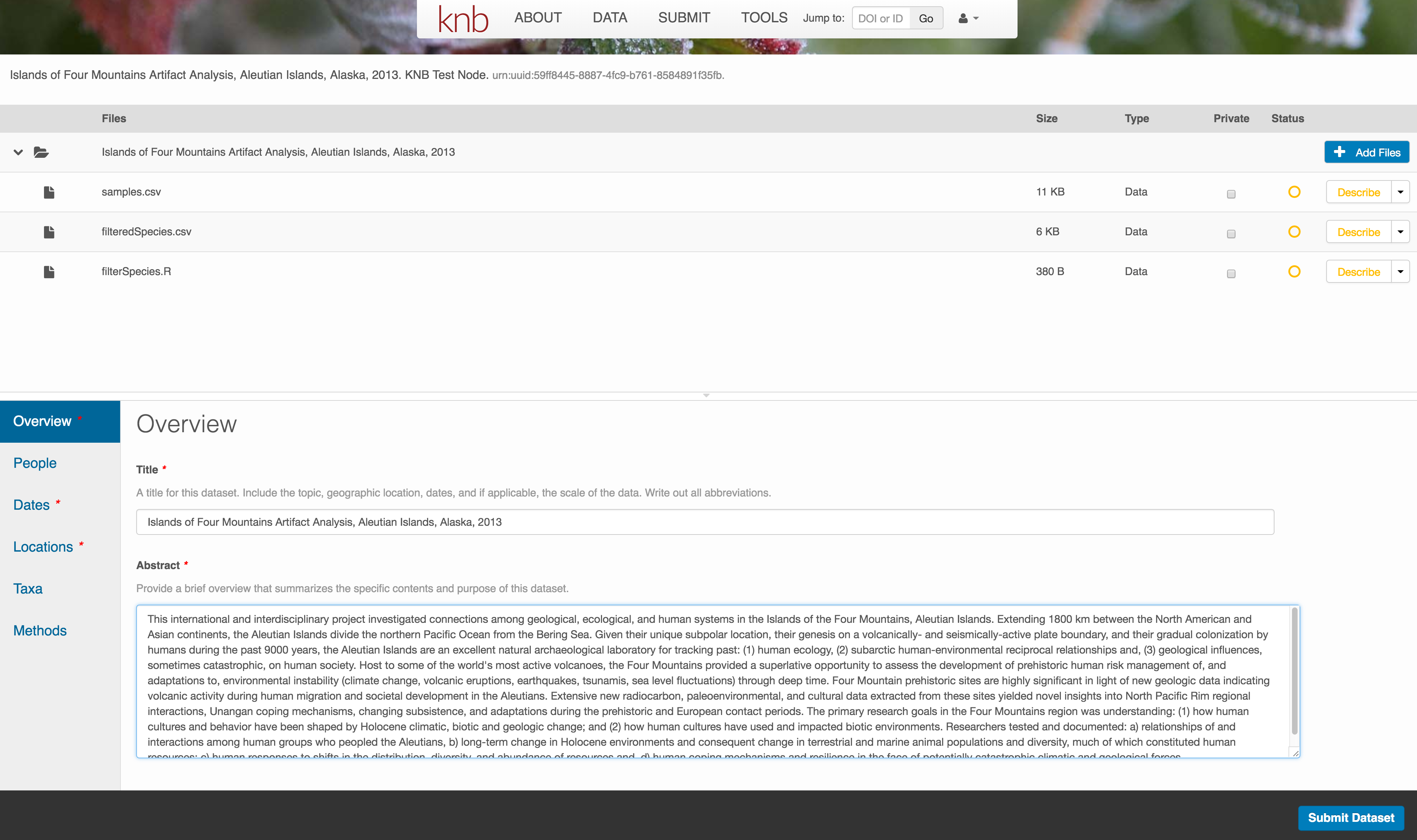
Enter Overview information
This includes a descriptive title, abstract, and keywords.
The title is the first way a potential user will get information about your dataset. It should be descriptive but succinct, lack acronyms, and include some indication of the temporal and geospatial coverage of the data.
The abstract should be sufficently descriptive for a general scientific audience to understand your dataset at a high level. It should provide an overview of the scientific context/project/hypotheses, how this data package fits into the larger context, a synopsis of the experimental or sampling design, and a summary of the data contents.
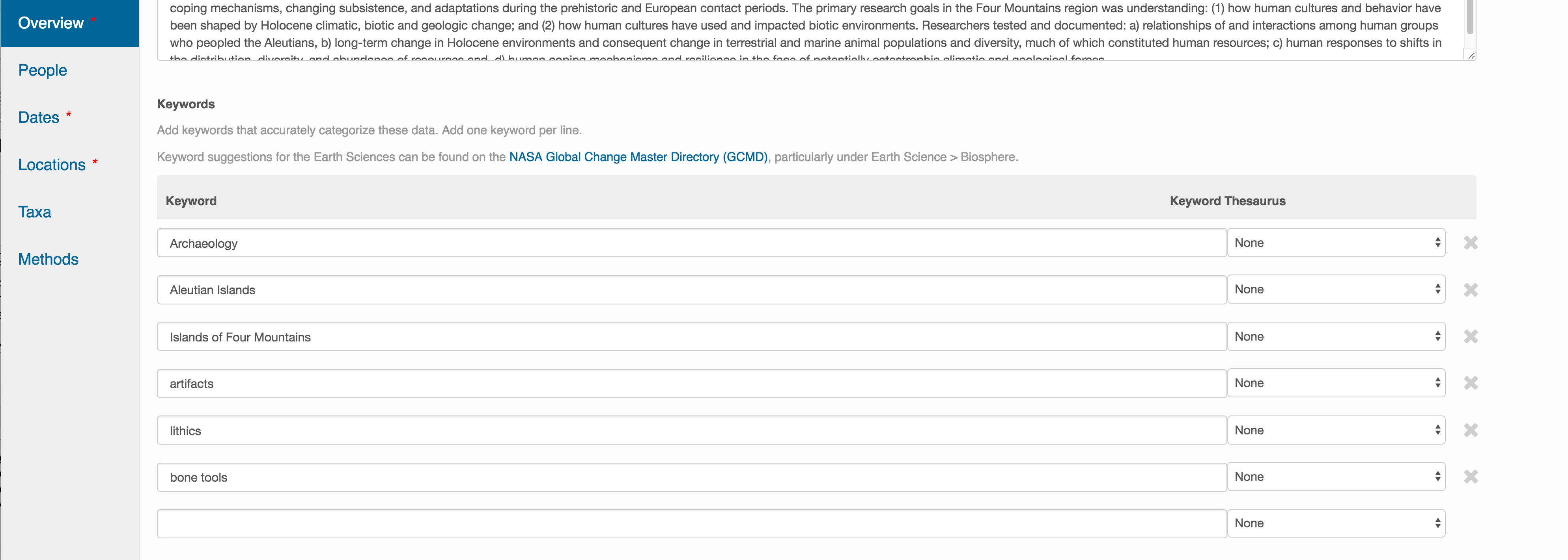
Keywords, while not required, can help increase the searchability of your dataset, particularly if they come from a semantically defined keyword thesaurus.
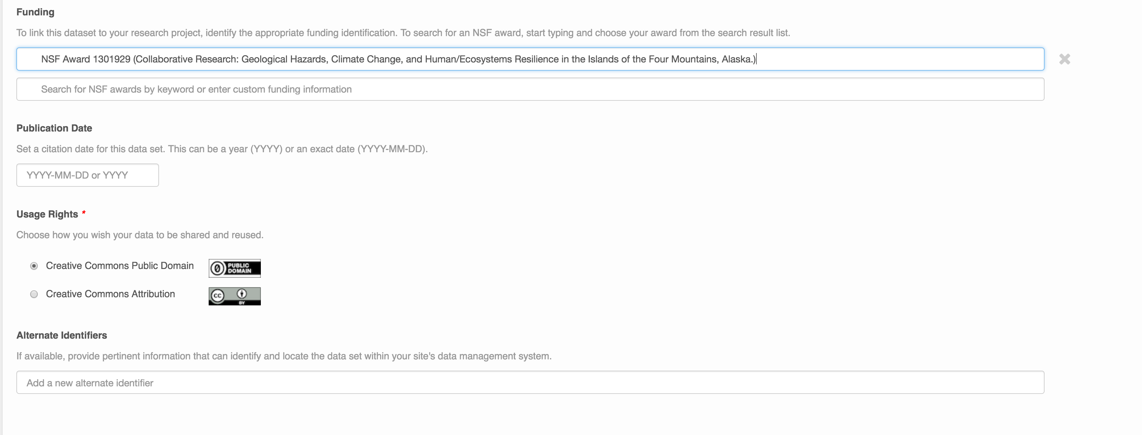
Optionally, you can also enter funding information, including a funding number, which can help link multiple datasets collected under the same grant.
Selecting a distribution license - either CC-0 or CC-BY is required.
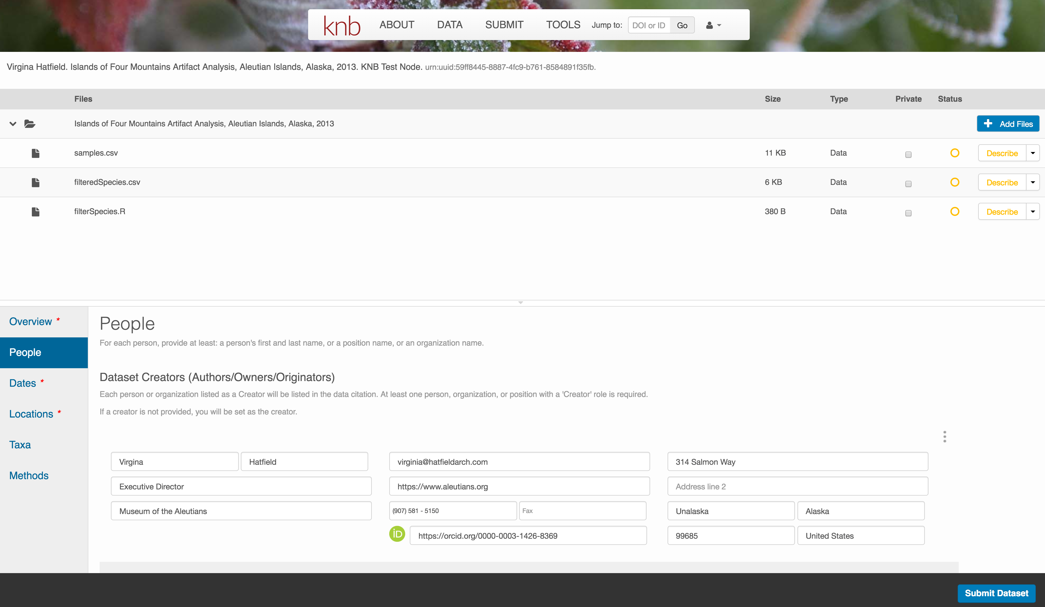
People Information
Information about the people associated with the dataset is essential to provide credit through citation and to help people understand who made contributions to the product. Enter information for the following people:
- Creators - all the people who should be in the citation for the dataset
- Contacts - one is required, but defaults to the first Creator if omitted
- Principal Investigators
- and any other that are relevant
For each, please strive to provide their ORCID identifier, which helps link this dataset to their other scholarly works.
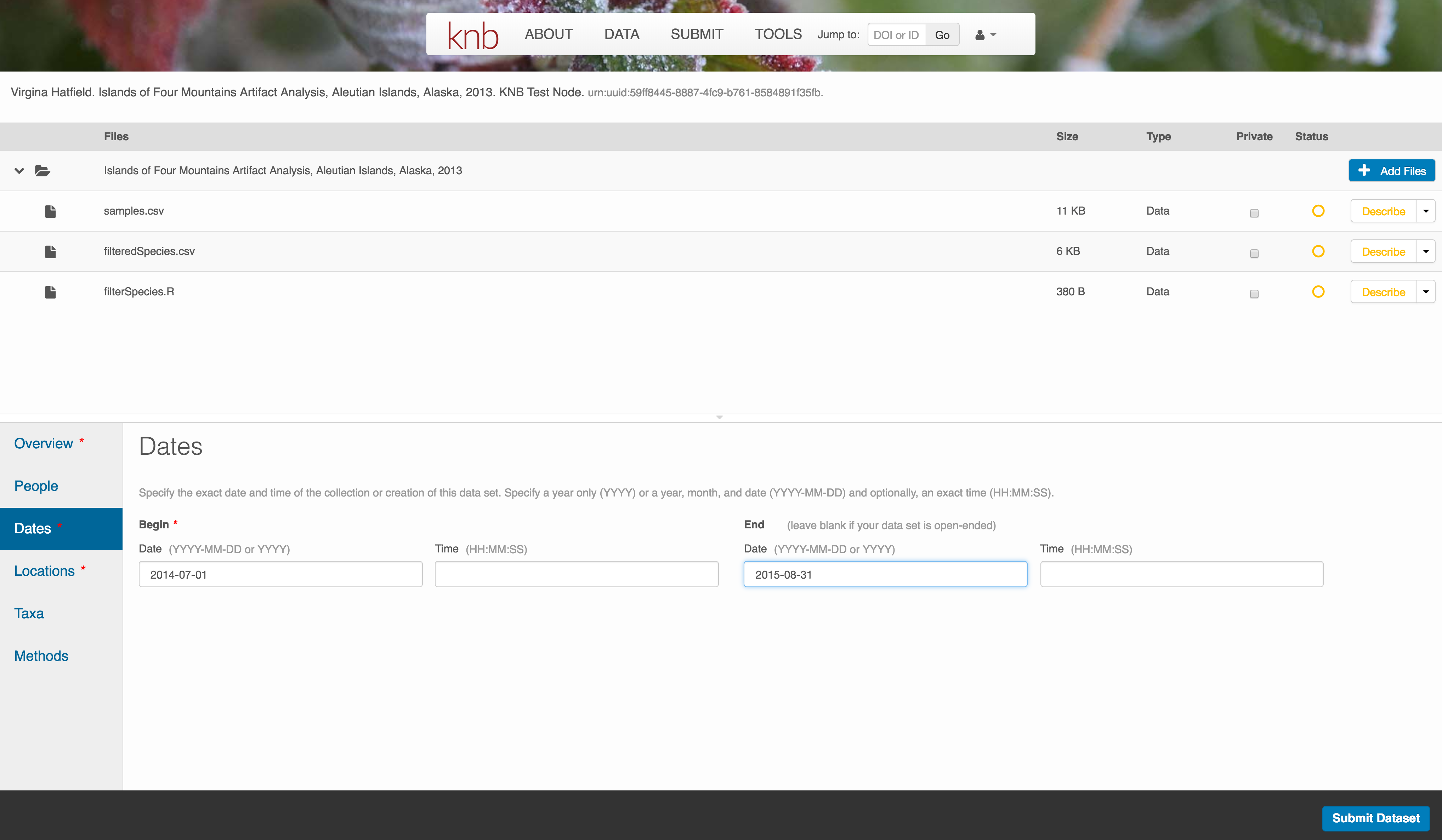
5.4.6.0.1 Temporal Information
Add the temporal coverage of the data, which represents the time period to which data apply.
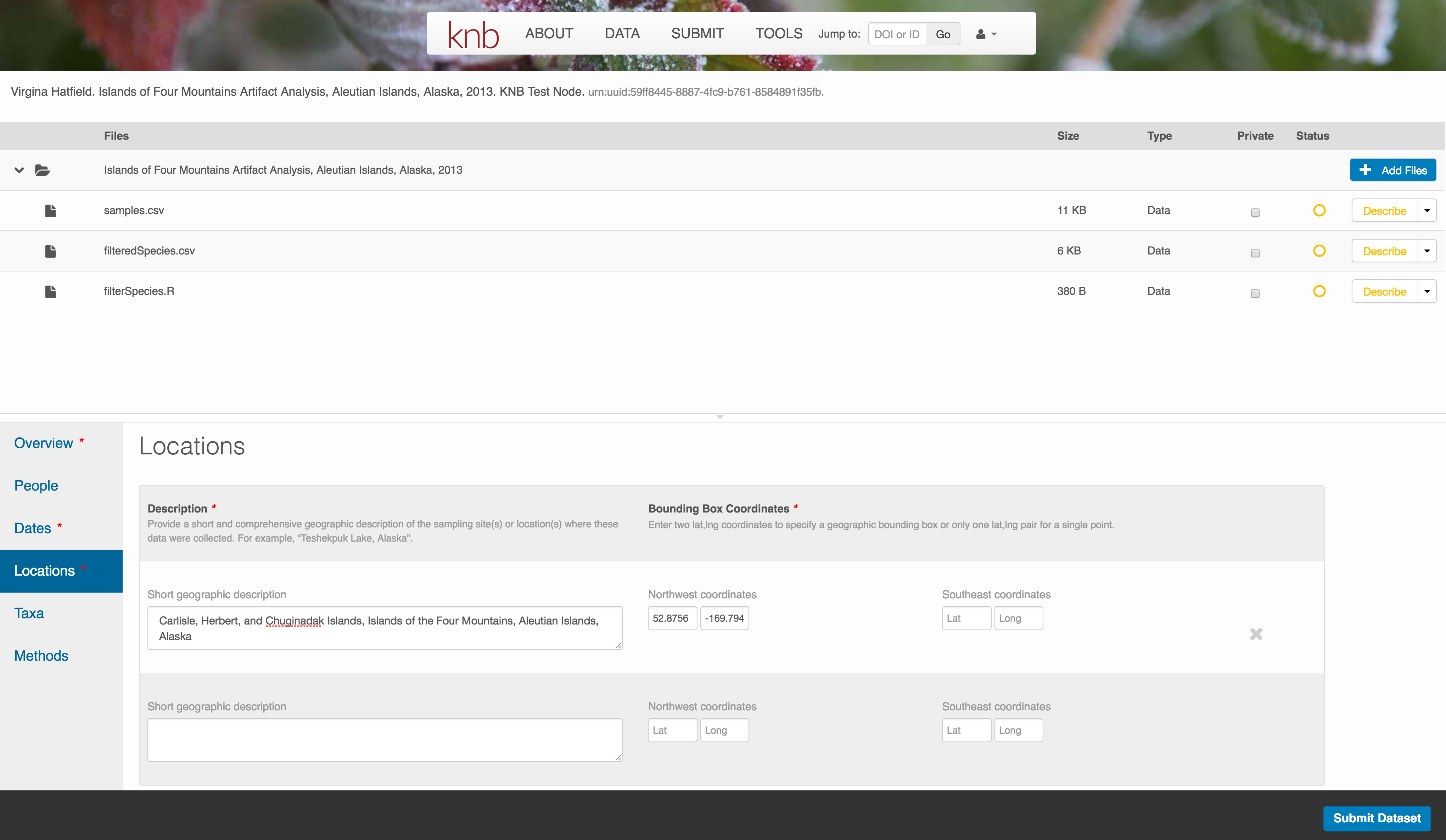
Location Information
The geospatial location that the data were collected is critical for discovery and interpretation of the data. Coordinates are entered in decimal degrees, and be sure to use negative values for West longitudes. The editor allows you to enter multiple locations, which you should do if you had noncontiguous sampling locations. This is particularly important if your sites are separated by large distances, so that a spatial search will be more precise.
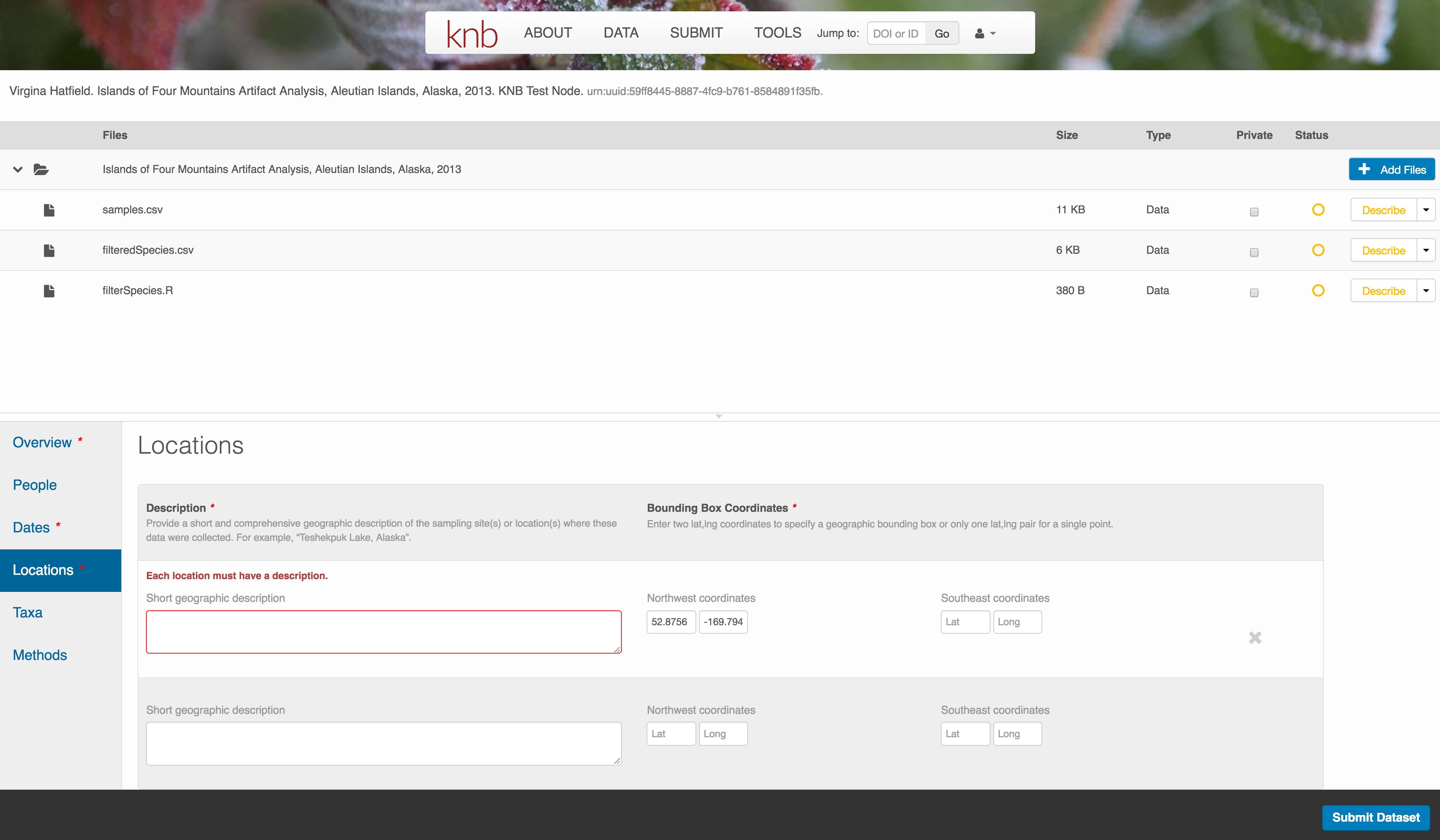
Note that, if you miss fields that are required, they will be highlighted in red to draw your attention. In this case, for the description, provide a comma-separated place name, ordered from the local to global. For example:
- Mission Canyon, Santa Barbara, California, USA
Methods
Methods are critical to accurate interpretation and reuse of your data. The editor allows you to add multiple different methods sections, include details of sampling methods, experimental design, quality assurance procedures, and computational techniques and software. Please be complete with your methods sections, as they are fundamentally important to reuse of the data.
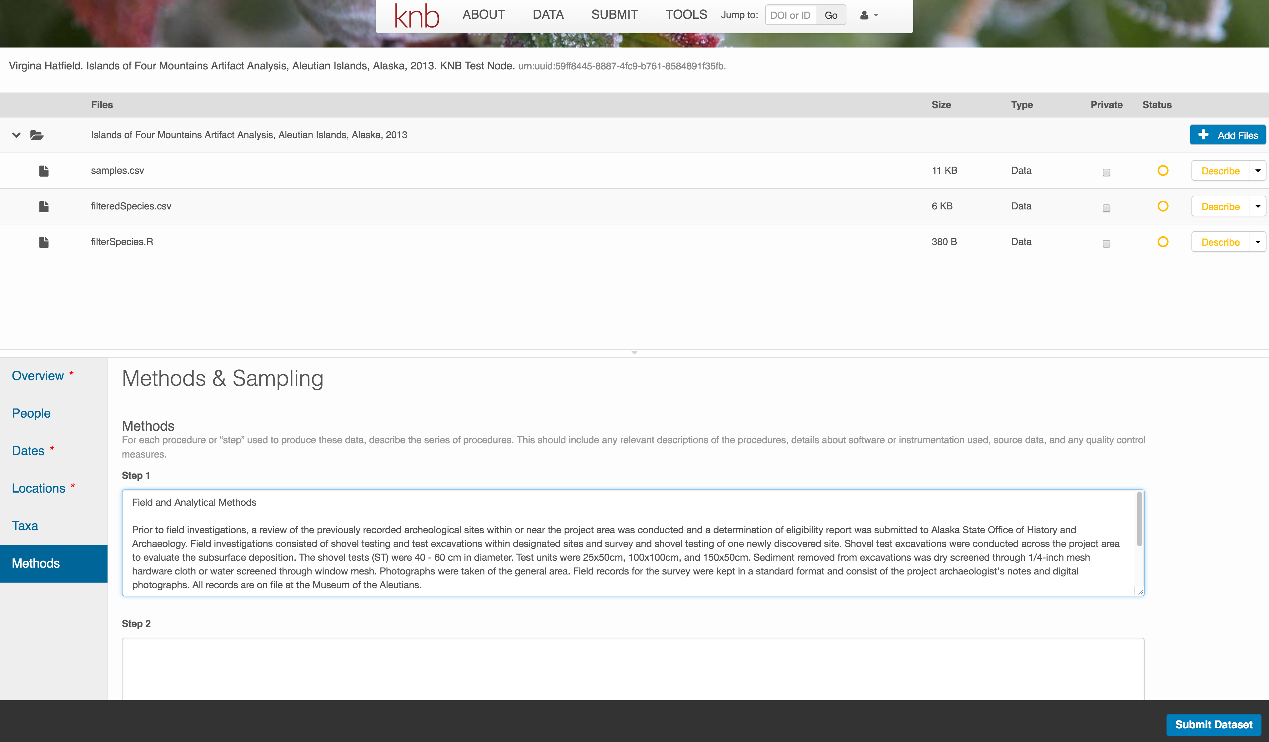
Save a first version with Submit
When finished, click the Submit Dataset button at the bottom.
If there are errors or missing fields, they will be highlighted.
Correct those, and then try submitting again. When you are successful, you should
see a green banner with a link to the current dataset view. Click the X
to close that banner, if you want to continue editing metadata.
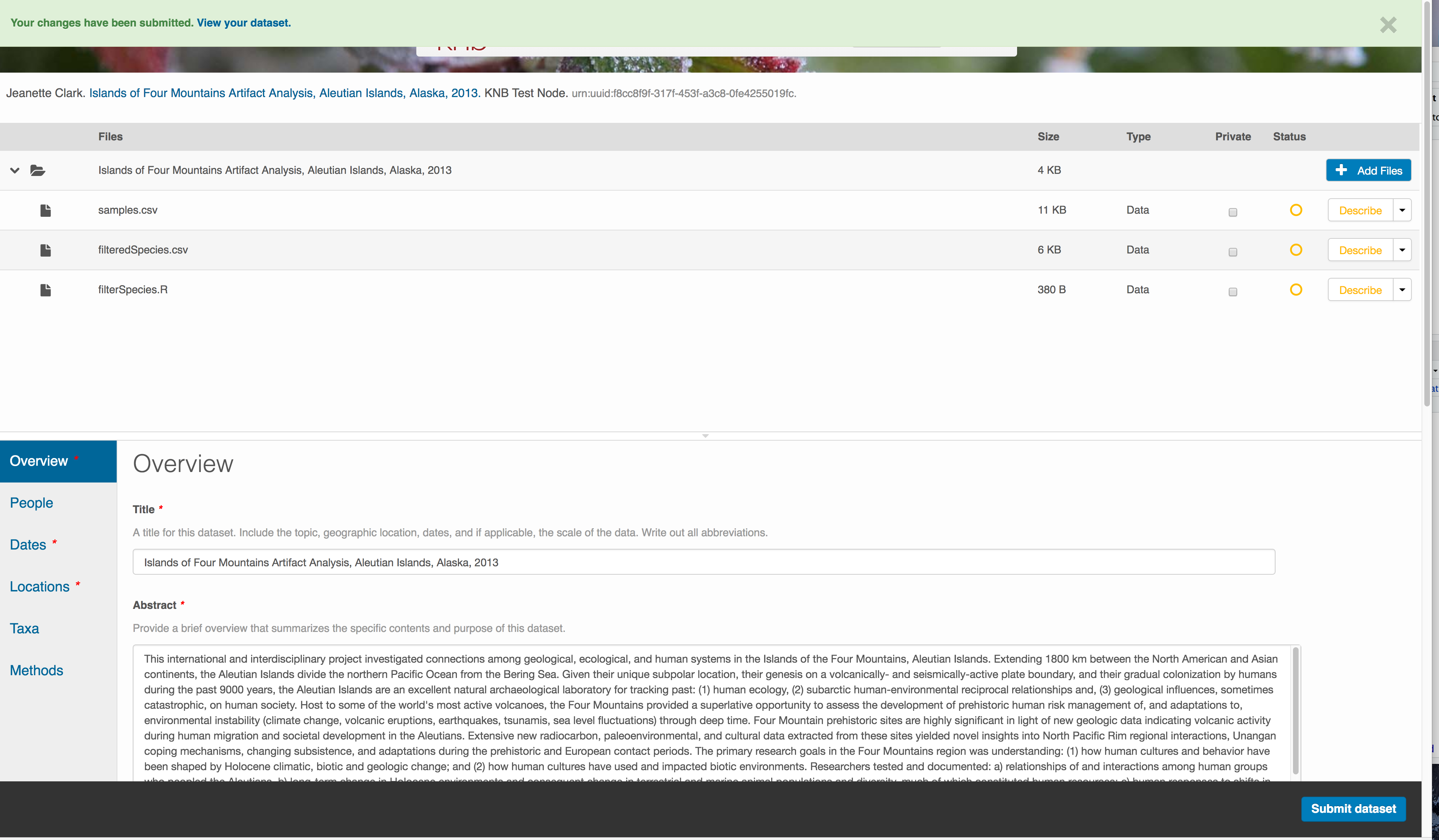
Success!
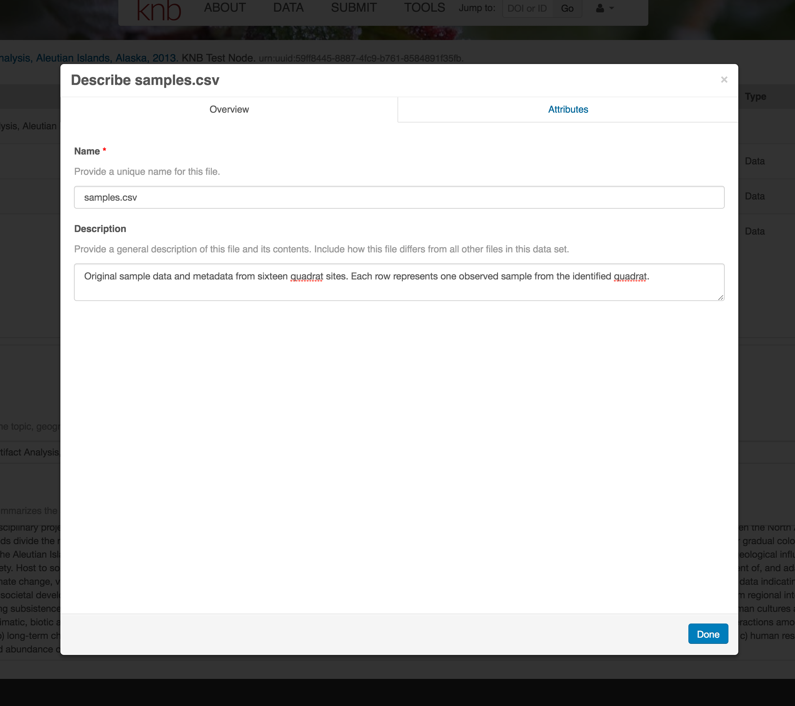
File and variable level metadata
The final major section of metadata concerns the structure and contents of your data files. In this case, provide the names and descriptions of the data contained in each file, as well as details of their internal structure.
For example, for data tables, you’ll need the name, label, and definition of each variable in your file. Click the Describe button to access a dialog to enter this information.
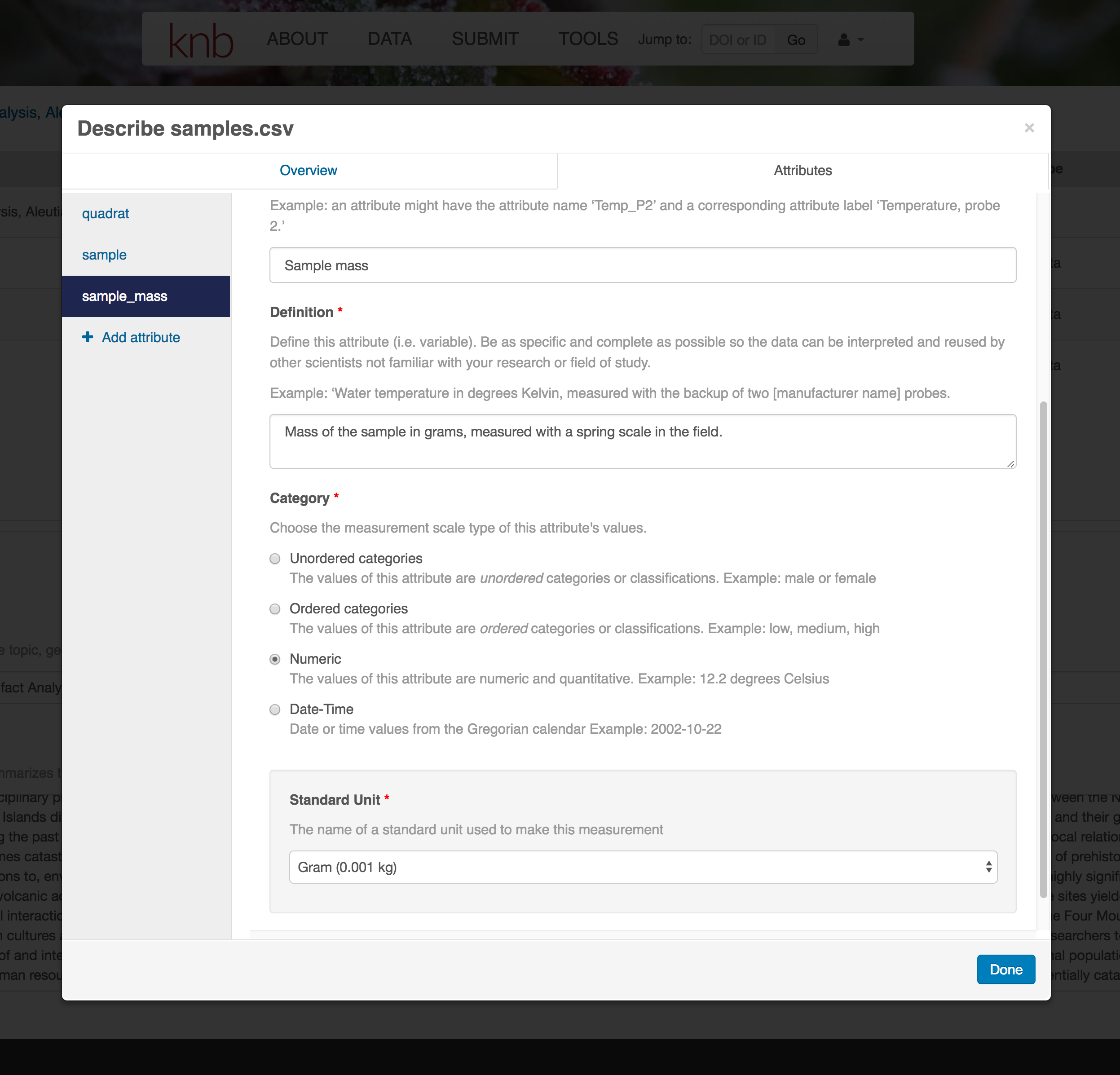
The Attributes tab is where you enter variable (aka attribute) information. In the case of tabular data (such as csv files) each column is an attribute, thus there should be one attribute defined for every column in your dataset. Attribute metadata includes:
- variable name (for programs)
- variable label (for display)
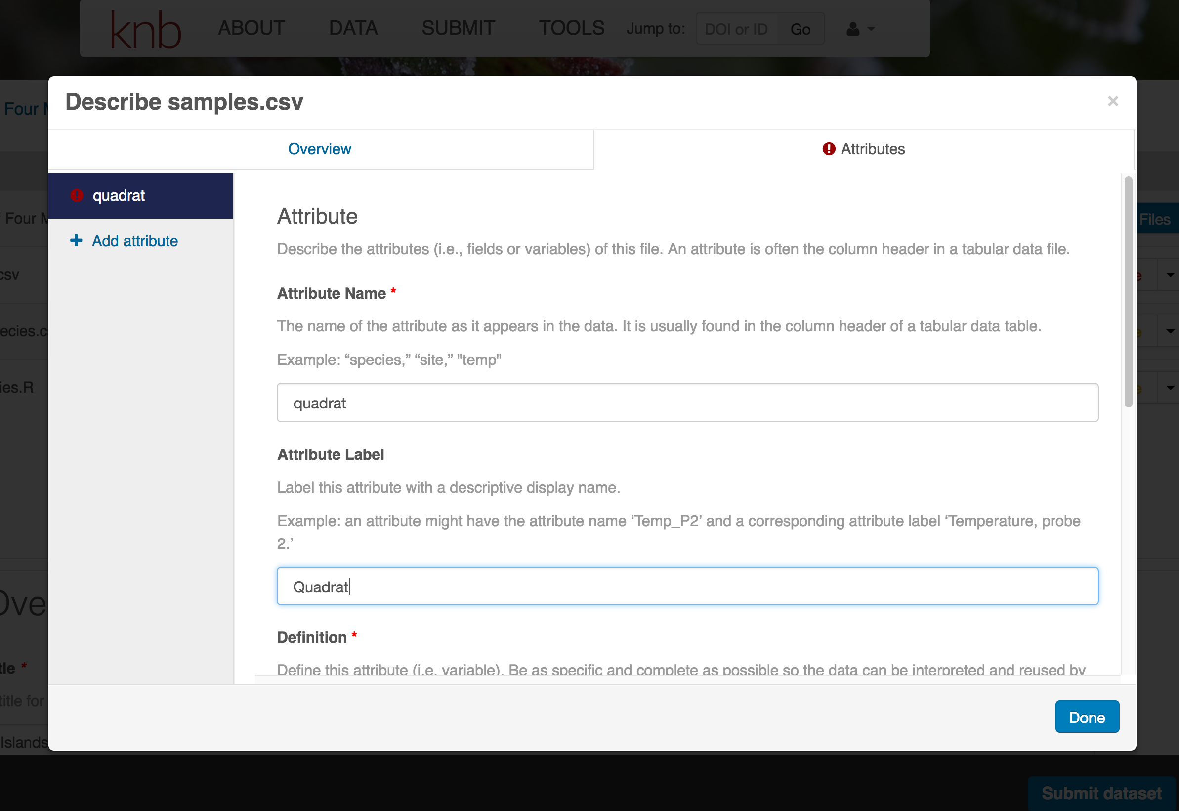
- variable definition (be specific)
- type of measurement
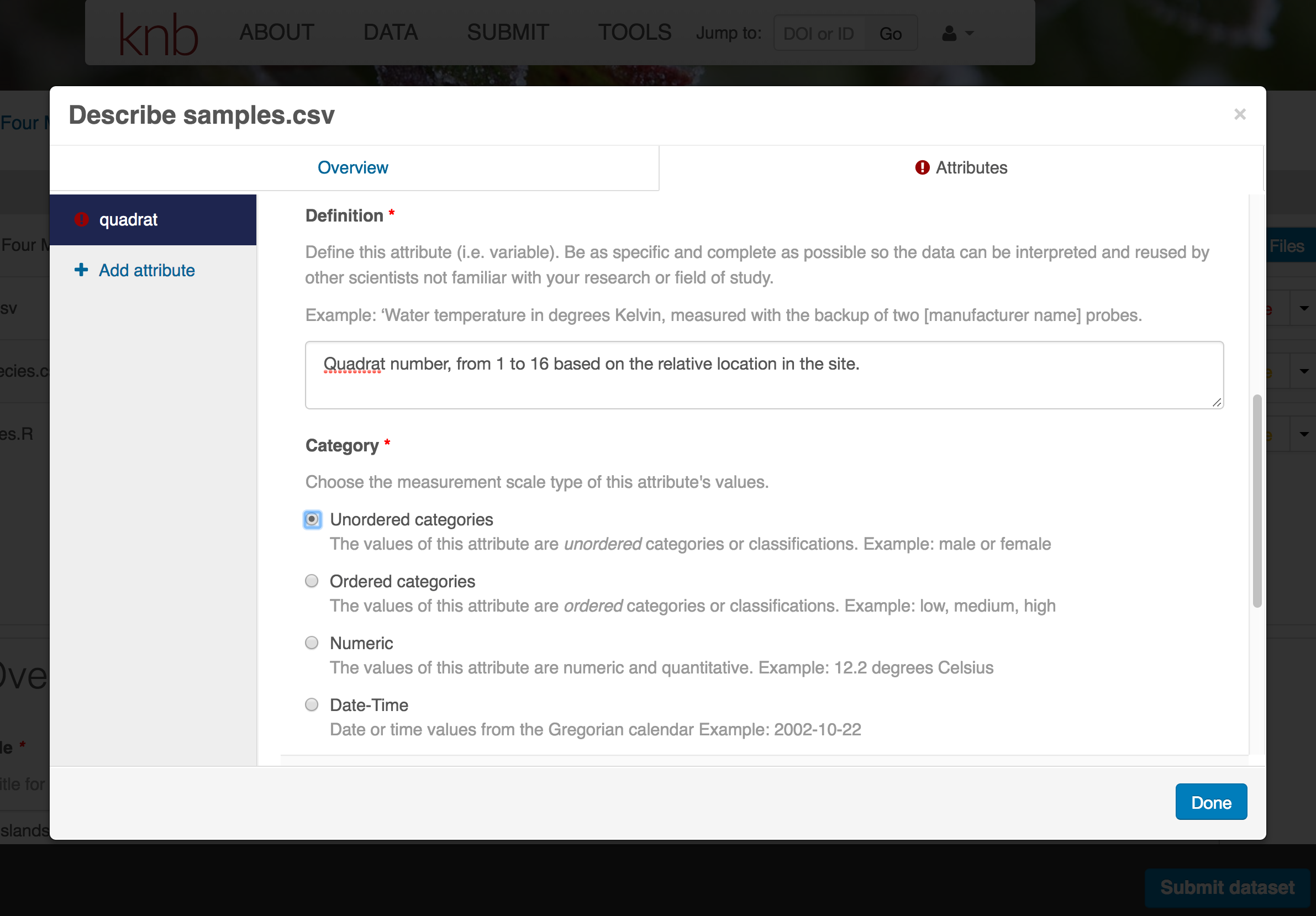
- units & code definitions
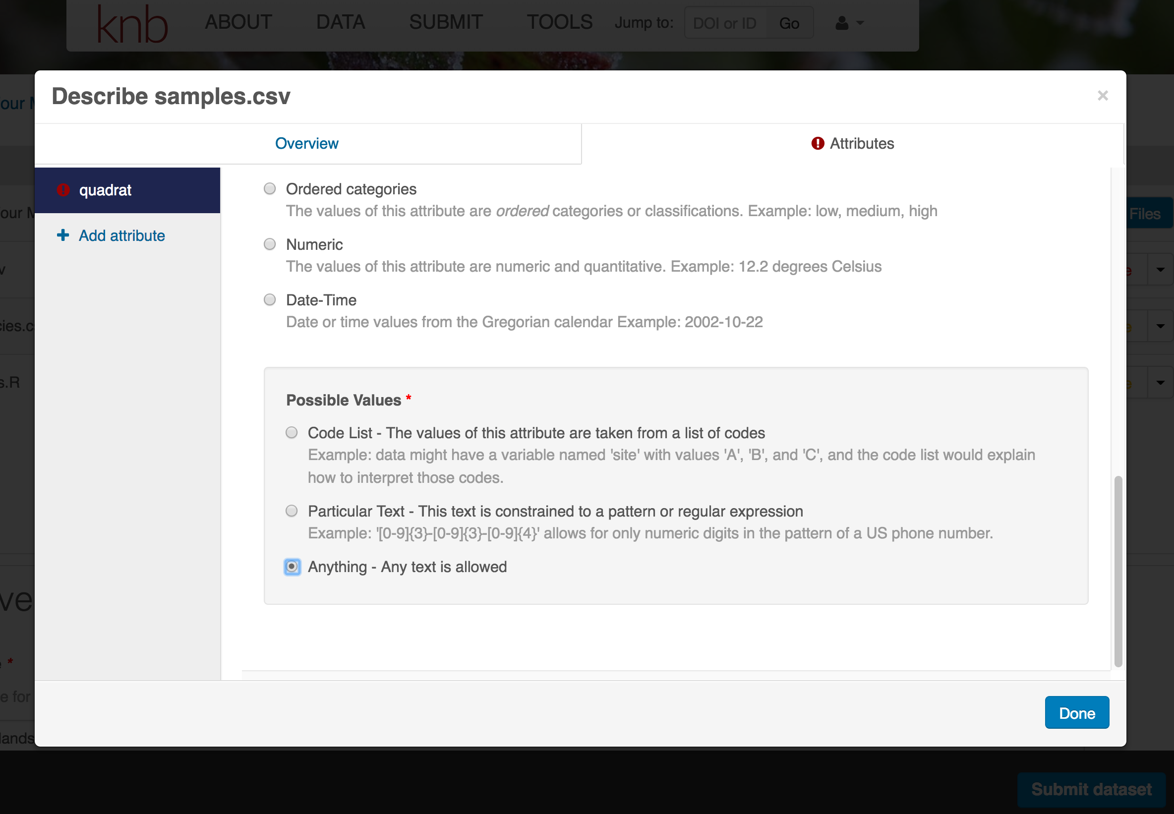
You’ll need to add these definitions for every variable (column) in the file. When done, click Done.
Now the list of data files will show a green checkbox indicating that you have full described that file’s internal structure. Proceed with the other CSV files, and then click Submit Dataset to save all of these changes.
Note that attribute information is not relevant for data files that do not contain variables, such as the R script in this example. Other examples of data files that might not need attributes are images, pdfs, and non-tabular text documents (such as readme files). The yellow circle in the editor indicates that attributes have not been filled out for a data file, and serves as a warning that they might be needed, depending on the file.
After you get the green success message, you can visit your dataset and review all of the information that you provided. If you find any errors, simply click Edit again to make changes.
Add workflow provenance
Understanding the relationships between files in a package is critically important, especially as the number of files grows. Raw data are transformed and integrated to produce derived data, that are often then used in analysis and visualization code to produce final outputs. In DataONE, we support structured descriptions of these relationships, so one can see the flow of data from raw data to derived to outputs.
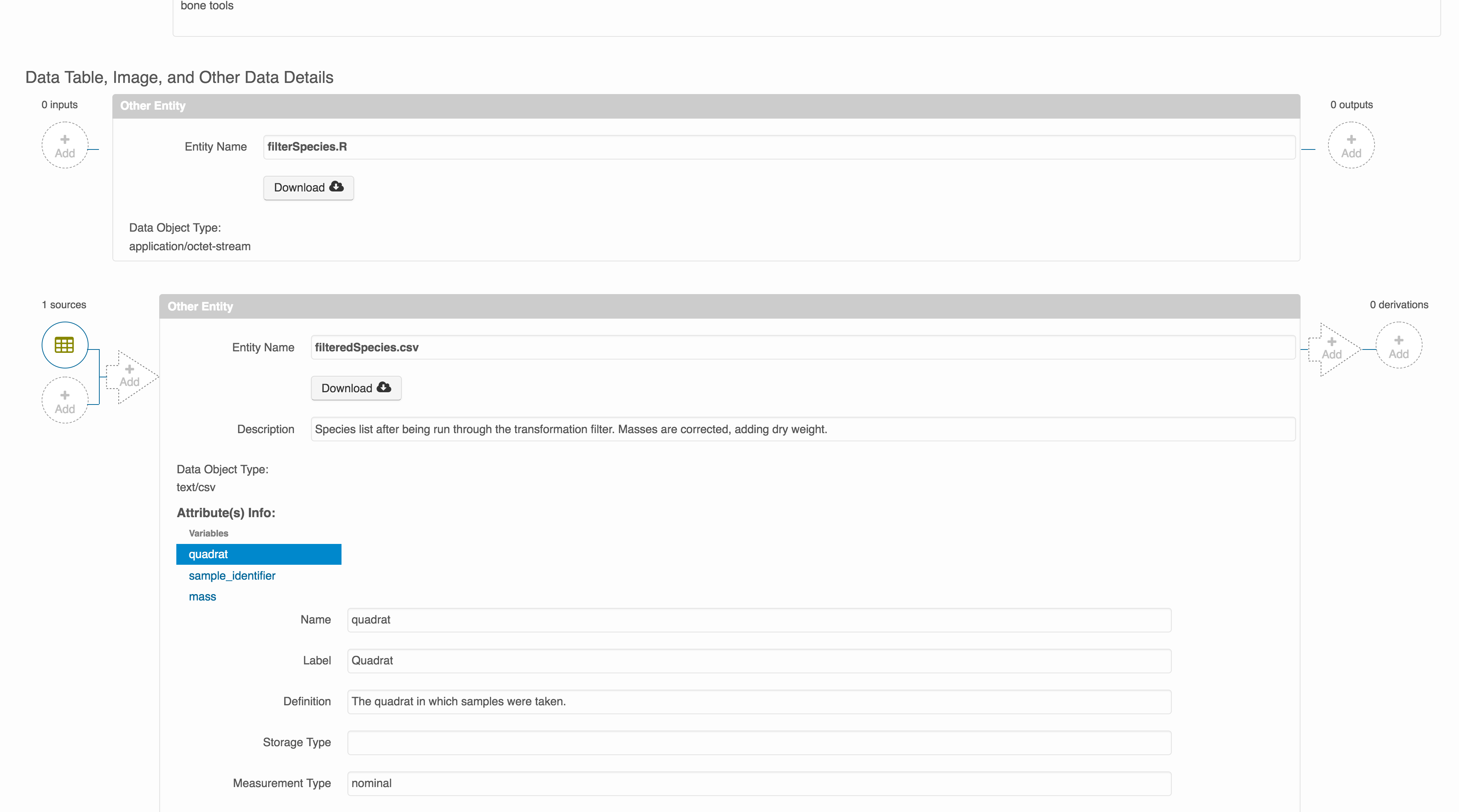
You add provenance by navigating to the data table descriptions, and selecting the
Add buttons to link the data and scripts that were used in your computational
workflow. On the left side, select the Add circle to add an input data source
to the filteredSpecies.csv file. This starts building the provenance graph to
explain the origin and history of each data object.
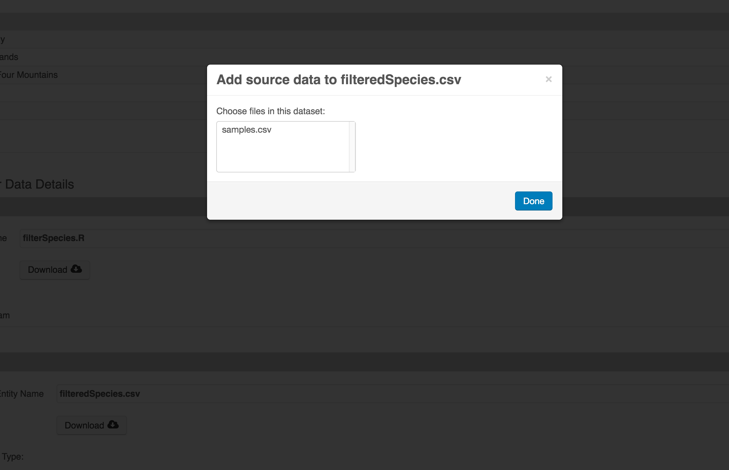
The linkage to the source dataset should appear.
Then you can add the link to the source code that handled the conversion
between the data files by clicking on Add arrow and selecting the R script:
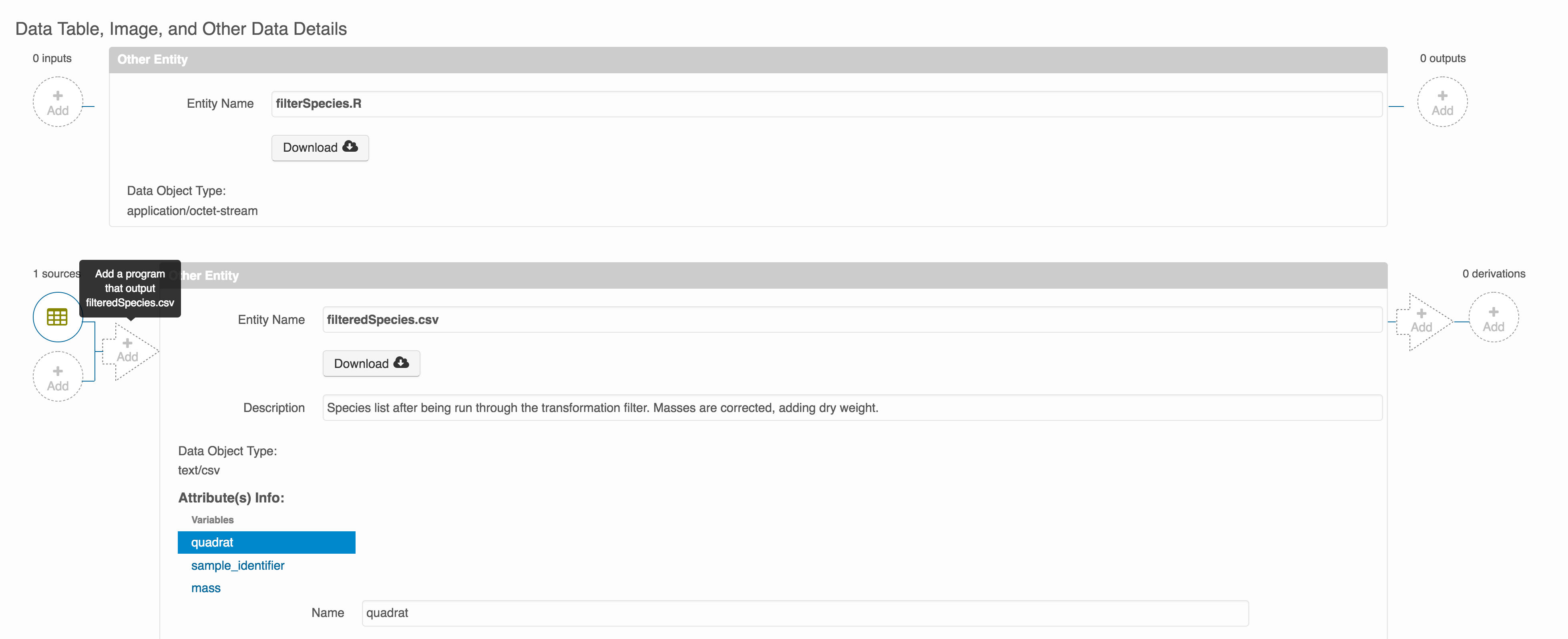
Select the R script and click “Done.”
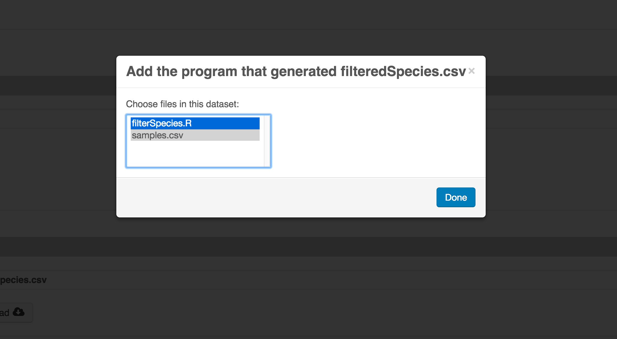
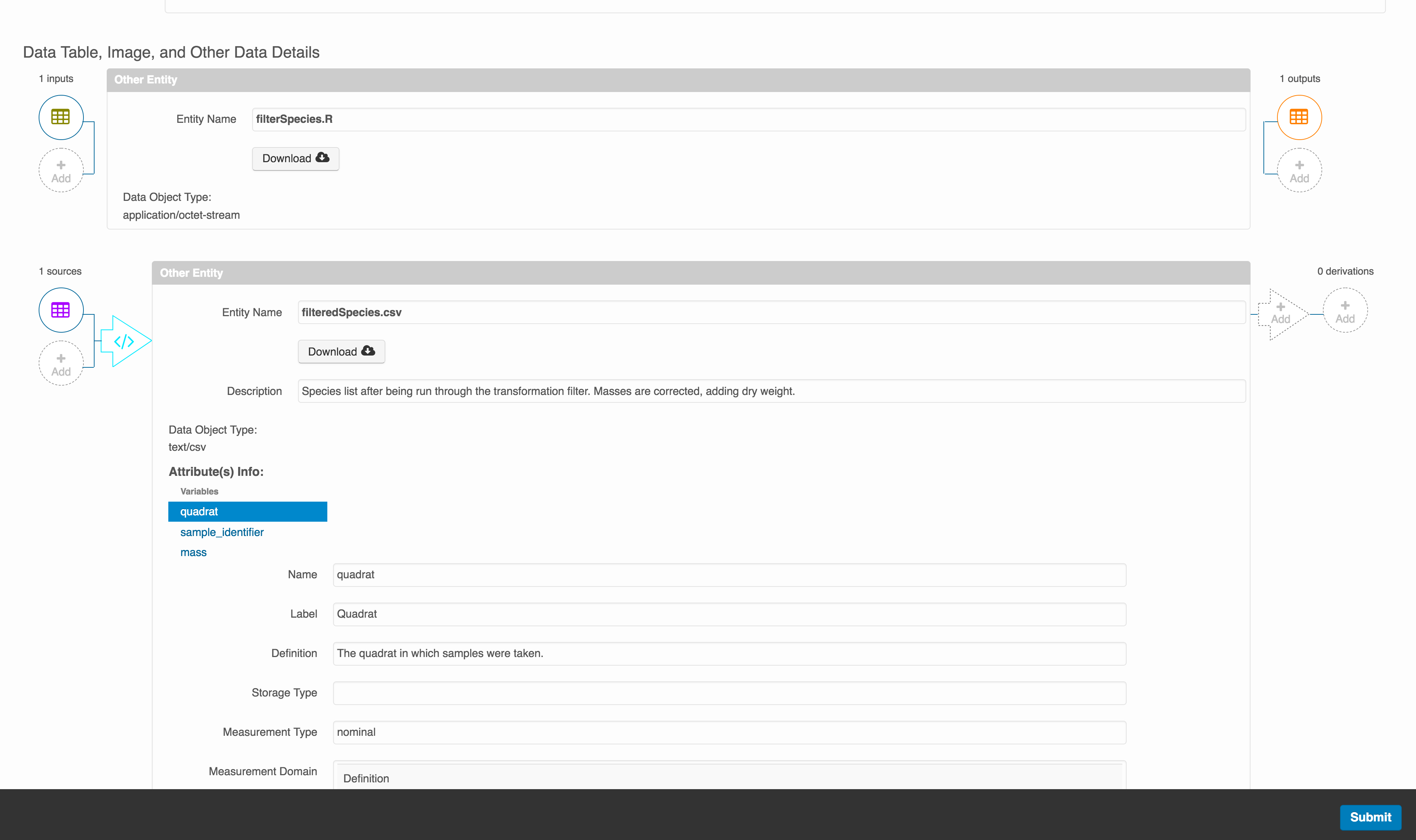
The diagram now shows the relationships among the data files and the R script, so click Submit to save another version of the package.
Et voilà! A beatifully preserved data package!
5.5 Introduction to R
5.5.1 Learning Objectives
In this lesson we will:
- get oriented to the RStudio interface
- work with R in the console
- be introduced to built-in R functions
- learn to use the help pages
5.5.2 Introduction and Motivation
There is a vibrant community out there that is collectively developing increasingly easy to use and powerful open source programming tools. The changing landscape of programming is making learning how to code easier than it ever has been. Incorporating programming into analysis workflows not only makes science more efficient, but also more computationally reproducible. In this course, we will use the programming language R, and the accompanying integrated development environment (IDE) RStudio. R is a great language to learn for data-oriented programming because it is widely adopted, user-friendly, and (most importantly) open source!
So what is the difference between R and RStudio? Here is an analogy to start us off. If you were a chef, R is a knife. You have food to prepare, and the knife is one of the tools that you’ll use to accomplish your task.
And if R were a knife, RStudio is the kitchen. RStudio provides a place to do your work! Other tools, communication, community, it makes your life as a chef easier. RStudio makes your life as a researcher easier by bringing together other tools you need to do your work efficiently - like a file browser, data viewer, help pages, terminal, community, support, the list goes on. So it’s not just the infrastructure (the user interface or IDE), although it is a great way to learn and interact with your variables, files, and interact directly with git. It’s also data science philosophy, R packages, community, and more. So although you can prepare food without a kitchen and we could learn R without RStudio, that’s not what we’re going to do. We are going to take advantage of the great RStudio support, and learn R and RStudio together.
Something else to start us off is to mention that you are learning a new language here. It’s an ongoing process, it takes time, you’ll make mistakes, it can be frustrating, but it will be overwhelmingly awesome in the long run. We all speak at least one language; it’s a similar process, really. And no matter how fluent you are, you’ll always be learning, you’ll be trying things in new contexts, learning words that mean the same as others, etc, just like everybody else. And just like any form of communication, there will be miscommunications that can be frustrating, but hands down we are all better off because of it.
While language is a familiar concept, programming languages are in a different context from spoken languages, but you will get to know this context with time. For example: you have a concept that there is a first meal of the day, and there is a name for that: in English it’s “breakfast”. So if you’re learning Spanish, you could expect there is a word for this concept of a first meal. (And you’d be right: ‘desayuno’). We will get you to expect that programming languages also have words (called functions in R) for concepts as well. You’ll soon expect that there is a way to order values numerically. Or alphabetically. Or search for patterns in text. Or calculate the median. Or reorganize columns to rows. Or subset exactly what you want. We will get you increase your expectations and learn to ask and find what you’re looking for.
5.5.2.1 Resources
This lesson is a combination of excellent lessons by others. Huge thanks to Julie Lowndes for writing most of this content and letting us build on her material, which in turn was built on Jenny Bryan’s materials. I definitely recommend reading through the original lessons and using them as reference:
Julie Lowndes’ Data Science Training for the Ocean Health Index
Jenny Bryan’s lectures from STAT545 at UBC
Here are some other resources that we like for learning R:
- Learn R in the console with swirl
- The Introduction to R lesson in Data Carpentry’s R for data analysis course
- The Stat 545 course materials
- The QCBS Introduction to R lesson (in French)
Other resources:
5.5.3 R at the console
Launch RStudio/R.
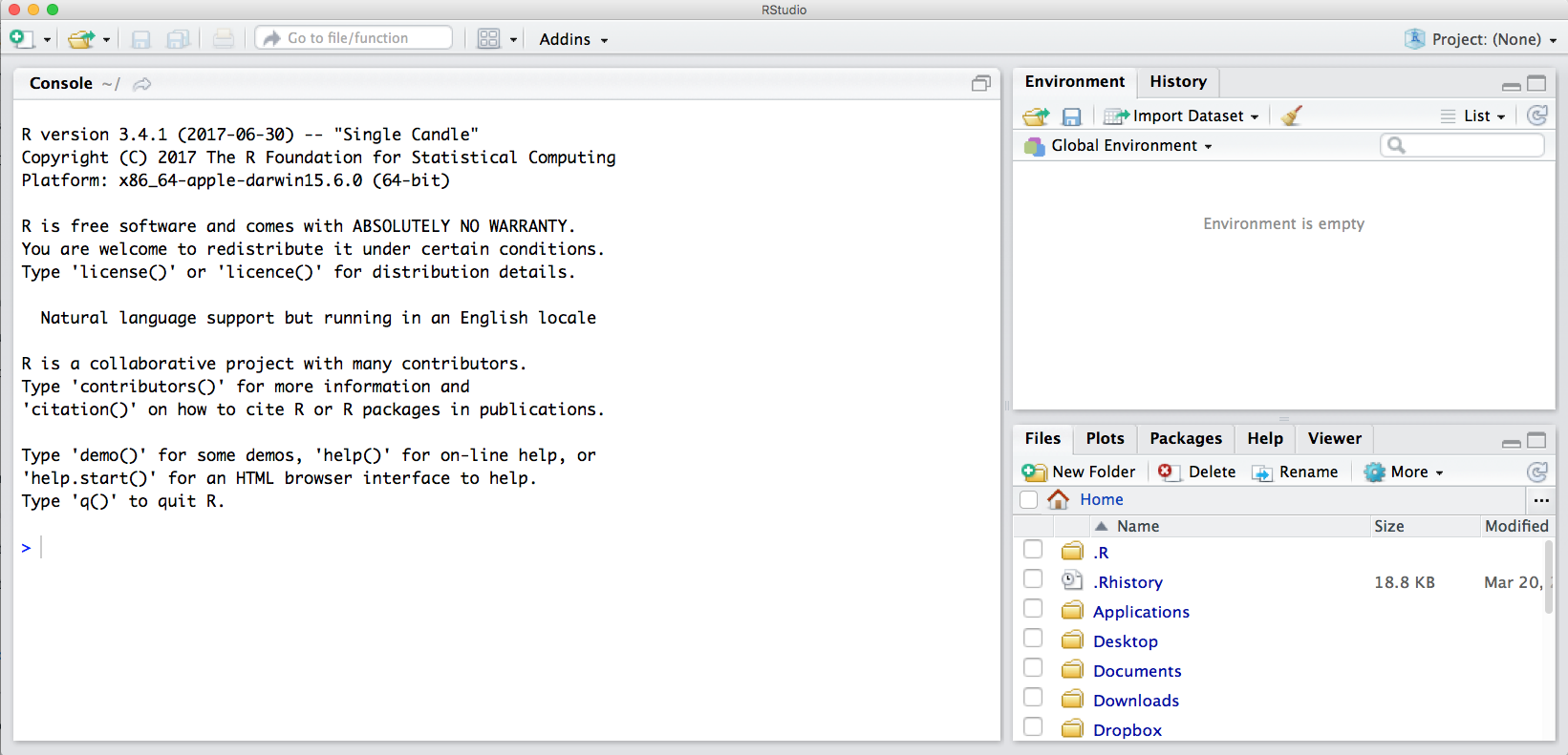
Notice the default panes:
- Console (entire left)
- Environment/History (tabbed in upper right)
- Files/Plots/Packages/Help (tabbed in lower right)
FYI: you can change the default location of the panes, among many other things: Customizing RStudio.
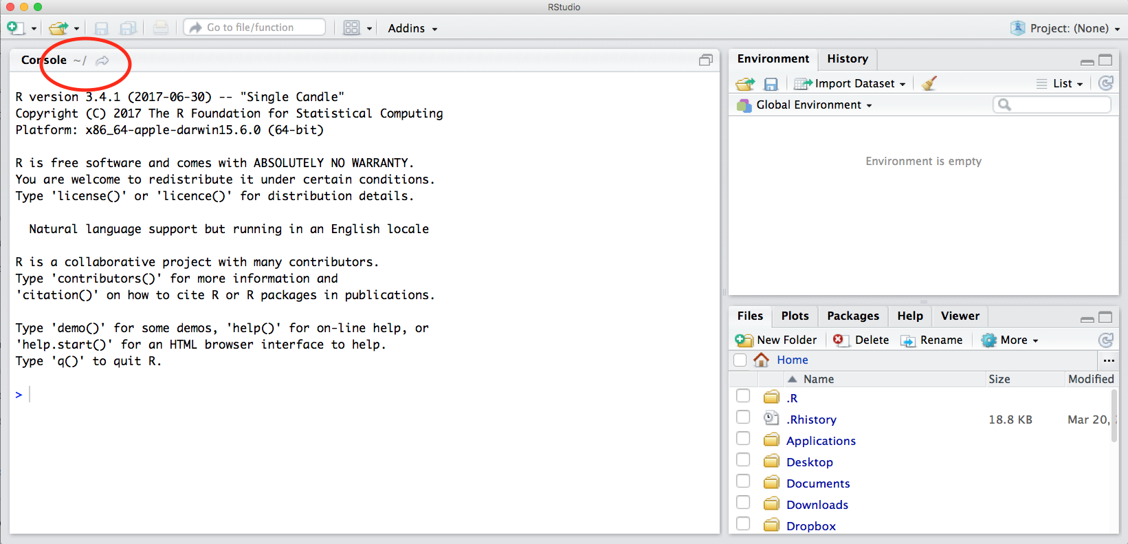
An important first question: where are we?
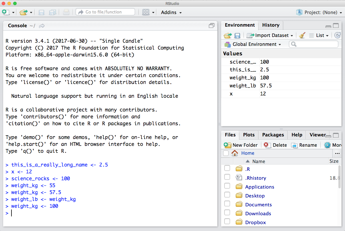
If you’ve just opened RStudio for the first time, you’ll be in your Home directory. This is noted by the ~/ at the top of the console. You can see too that the Files pane in the lower right shows what is in the Home directory where you are. You can navigate around within that Files pane and explore, but note that you won’t change where you are: even as you click through you’ll still be Home: ~/.
OK let’s go into the Console, where we interact with the live R process.
We use R to calculate things for us, so let’s do some simple math.
## [1] 12You can assign the value of that mathematic operation to a variable, or object, in R. You do this using the assignment operator, <-.
Make an assignment and then inspect the object you just created.
## [1] 12In my head I hear, e.g., “x gets 12”.
All R statements where you create objects – “assignments” – have this form: objectName <- value.
I’ll write it in the console with a hash #, which is the way R comments so it won’t be evaluated.
## objectName <- value

## This is also how you write notes in your code to explain what you are doing.
Object names cannot start with a digit and cannot contain certain other characters such as a comma or a space. You will be wise to adopt a convention for demarcating words in names.
Make an assignment
To inspect this variable, instead of typing it, we can press the up arrow key and call your command history, with the most recent commands first. Let’s do that, and then delete the assignment:
## [1] 2.5Another way to inspect this variable is to begin typing this_…and RStudio will automagically have suggested completions for you that you can select by hitting the tab key, then press return.
One more:
You can see that we can assign an object to be a word, not a number. In R, this is called a “string”, and R knows it’s a word and not a number because it has quotes " ". You can work with strings in your data in R pretty easily, thanks to the stringr and tidytext packages. We won’t talk about strings very much specifically, but know that R can handle text, and it can work with text and numbers together.
Strings and numbers lead us to an important concept in programming: that there are different “classes” or types of objects. An object is a variable, function, data structure, or method that you have written to your environment. You can see what objects you have loaded by looking in the “environment” pane in RStudio. The operations you can do with an object will depend on what type of object it is. This makes sense! Just like you wouldn’t do certain things with your car (like use it to eat soup), you won’t do certain operations with character objects (strings), for example.
Try running the following line in your console:
What happened? Why?
You may have noticed that when assigning a value to an object, R does not print anything. You can force R to print the value by using parentheses or by typing the object name:
weight_kg <- 55    # doesn't print anything
(weight_kg <- 55)  # but putting parenthesis around the call prints the value of `weight_kg`
## [1] 55## [1] 55Now that R has weight_kg in memory, we can do arithmetic with it. For instance, we may want to convert this weight into pounds (weight in pounds is 2.2 times the weight in kg):
## [1] 121We can also change a variable’s value by assigning it a new one:
## [1] 126.5This means that assigning a value to one variable does not change the values of other variables. For example, let’s store the animal’s weight in pounds in a new variable, weight_lb:
and then change weight_kg to 100.
What do you think is the current content of the object weight_lb? 126.5 or 220? Why?
You can also store more than one value in a single object. Storing a series of weights in a single object is a convenient way to perform the same operation on multiple values at the same time. One way to create such an object is the function c(), which stands for combine or concatenate.
Here we will create a vector of weights in kilograms, and convert them to pounds, saving the weight in pounds as a new object.
## [1] 55 25 12## [1] 121.0 55.0 26.45.5.3.1 Error messages are your friends
Implicit contract with the computer/scripting language: Computer will do tedious computation for you. In return, you will be completely precise in your instructions. Typos matter. Case matters. Pay attention to how you type.
Remember that this is a language, not unsimilar to English! There are times you aren’t understood – it’s going to happen. There are different ways this can happen. Sometimes you’ll get an error. This is like someone saying ‘What?’ or ‘Pardon’? Error messages can also be more useful, like when they say ‘I didn’t understand this specific part of what you said, I was expecting something else’. That is a great type of error message. Error messages are your friend. Google them (copy-and-paste!) to figure out what they mean.
And also know that there are errors that can creep in more subtly, without an error message right away, when you are giving information that is understood, but not in the way you meant. Like if I’m telling a story about tables and you’re picturing where you eat breakfast and I’m talking about data. This can leave me thinking I’ve gotten something across that the listener (or R) interpreted very differently. And as I continue telling my story you get more and more confused… So write clean code and check your work as you go to minimize these circumstances!
5.5.3.2 Logical operators and expressions
A moment about logical operators and expressions. We can ask questions about the objects we just made.
==means ‘is equal to’!=means ‘is not equal to’<means ` is less than’>means ` is greater than’<=means ` is less than or equal to’>=means ` is greater than or equal to’
## [1] FALSE FALSE FALSE## [1] TRUE FALSE FALSE## [1] TRUE TRUE TRUEShortcuts You will make lots of assignments and the operator
<-is a pain to type. Don’t be lazy and use=, although it would work, because it will just sow confusion later. Instead, utilize RStudio’s keyboard shortcut: Alt + - (the minus sign). Notice that RStudio automagically surrounds<-with spaces, which demonstrates a useful code formatting practice. Code is miserable to read on a good day. Give your eyes a break and use spaces. RStudio offers many handy keyboard shortcuts. Also, Alt+Shift+K brings up a keyboard shortcut reference card.
5.5.3.3 Clearing the environment
Now look at the objects in your environment (workspace) – in the upper right pane. The workspace is where user-defined objects accumulate.
You can also get a listing of these objects with a few different R commands:
## [1] "science_rocks"
## [2] "this_is_a_really_long_name"
## [3] "weight_kg"
## [4] "weight_lb"
## [5] "x"## [1] "science_rocks"
## [2] "this_is_a_really_long_name"
## [3] "weight_kg"
## [4] "weight_lb"
## [5] "x"If you want to remove the object named weight_kg, you can do this:
To remove everything:
or click the broom in RStudio’s Environment pane.
5.5.4 R functions, help pages
So far we’ve learned some of the basic syntax and concepts of R programming, and how to navigate RStudio, but we haven’t done any complicated or interesting programming processes yet. This is where functions come in!
A function is a way to group a set of commands together to undertake a task in a reusable way. When a function is executed, it produces a return value. We often say that we are “calling” a function when it is executed. Functions can be user defined and saved to an object using the assignment operator, so you can write whatever functions you need, but R also has a mind-blowing collection of built-in functions ready to use. To start, we will be using some built in R functions.
All functions are called using the same syntax: function name with parentheses around what the function needs in order to do what it was built to do. The pieces of information that the function needs to do its job are called arguments. So the syntax will look something like: result_value <- function_name(argument1 = value1, argument2 = value2, ...).
5.5.4.1 A simple example
To take a very simple example, let’s look at the mean() function. As you might expect, this is a function that will take the mean of a set of numbers. Very convenient!
Let’s create our vector of weights again:
and use the mean function to calculate the mean weight.
## [1] 30.666675.5.4.2 Getting help
What if you know the name of the function that you want to use, but don’t know exactly how to use it? Thankfully RStudio provides an easy way to access the help documentation for functions.
To access the help page for mean, enter the following into your console:
The help pane will show up in the lower right hand corner of your RStudio.
The help page is broken down into sections:
- Description: An extended description of what the function does.
- Usage: The arguments of the function(s) and their default values.
- Arguments: An explanation of the data each argument is expecting.
- Details: Any important details to be aware of.
- Value: The data the function returns.
- See Also: Any related functions you might find useful.
- Examples: Some examples for how to use the function.
5.5.4.3 Your turn
Exercise: Look up the help file for a function that you know or expect to exist. Here are some ideas:
?getwd(),?plot(),min(),max(),?log()).
And there’s also help for when you only sort of remember the function name: double-questionmark:
Not all functions have (or require) arguments:
## [1] "Tue Feb 16 11:53:44 2021"5.6 Literate Analysis with RMarkdown
5.6.1 Learning Objectives
In this lesson we will:
- explore an example of RMarkdown as literate analysis
- learn markdown syntax
- write and run R code in RMarkdown
- build and knit an example document
5.6.2 Introduction and motivation
The concept of literate analysis dates to a 1984 article by Donald Knuth. In this article, Knuth proposes a reversal of the programming paradigm.
Instead of imagining that our main task is to instruct a computer what to do, let us concentrate rather on explaining to human beings what we want a computer to do.
If our aim is to make scientific research more transparent, the appeal of this paradigm reversal is immediately apparent. All too often, computational methods are written in such a way as to be borderline incomprehensible - even to the person who originally wrote the code! The reason for this is obvious, computers interpret information very differently than people do. By switching to a literate analysis model, you help enable human understanding of what the computer is doing. As Knuth describes, in the literate analysis model, the author is an “essayist” who chooses variable names carefully, explains what they mean, and introduces concepts in the analysis in a way that facilitates understanding.
RMarkdown is an excellent way to generate literate analysis, and a reproducible workflow. RMarkdown is a combination of two things - R, the programming language, and markdown, a set of text formatting directives. In R, the language assumes that you are writing R code, unless you specify that you are writing prose (using a comment, designated by #). The paradigm shift of literate analysis comes in the switch to RMarkdown, where instead of assuming you are writing code, Rmarkdown assumes that you are writing prose unless you specify that you are writing code. This, along with the formatting provided by markdown, encourages the “essayist” to write understandable prose to accompany the code that explains to the human-beings reading the document what the author told the computer to do. This is in contrast to writing just R code, where the author telling to the computer what to do with maybe a smattering of terse comments explaining the code to a reader.
Before we dive in deeper, let’s look at an example of what literate analysis with RMarkdown can look like using a real example. Here is an example of a real analysis workflow written using RMarkdown.
There are a few things to notice about this document, which assembles a set of similar data sources on salmon brood tables with different formatting into a single data source.
- It introduces the data sources using in-line images, links, interactive tables, and interactive maps.
- An example of data formatting from one source using R is shown.
- The document executes a set of formatting scripts in a directory to generate a single merged file.
- Some simple quality checks are performed (and their output shown) on the merged data.
- Simple analysis and plots are shown.
In addition to achieving literate analysis, this document also represents a reproducible analysis. Because the entire merging and quality control of the data is done using the R code in the RMarkdown, if a new data source and formatting script are added, the document can be run all at once with a single click to re-generate the quality control, plots, and analysis of the updated data.
RMarkdown is an amazing tool to use for collaborative research, so we will spend some time learning it well now, and use it through the rest of the course.
Setup
Open a new RMarkdown file using the following prompts:
File -> New File -> RMarkdown
A popup window will appear. You can just click the OK button here, or give your file a new title if you wish. Leave the output format as HTML.
5.6.3 Basic RMarkdown syntax
The first thing to notice is that by opening a file, we are seeing the 4th pane of the RStudio console, which is essentially a text editor.
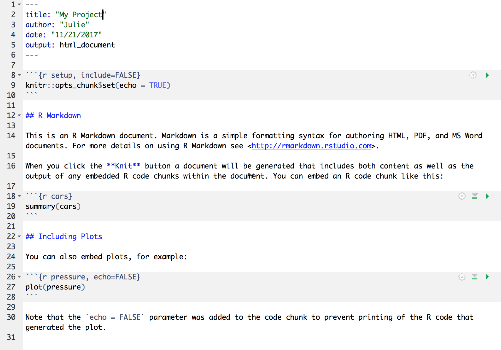
Let’s have a look at this file — it’s not blank; there is some initial text already provided for you. Notice a few things about it:
- There are white and grey sections. R code is in grey sections, and other text is in white.
Let’s go ahead and “Knit” the document by clicking the blue yarn at the top of the RMarkdown file. When you first click this button, RStudio will prompt you to save this file. Save it in the top level of your home directory on the server, and name it something that you will remember (like rmarkdown-intro.Rmd).
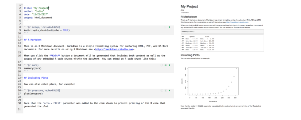
What do you notice between the two?
First, the knit process produced a second file (an HTML file) that popped up in a second window. You’ll also see this file in your directory with the same name as your Rmd, but with the html extension. In it’s simplest format, RMarkdown files come in pairs - the RMarkdown file, and its rendered version. In this case, we are knitting, or rendering, the file into HTML. You can also knit to PDF or Word files.
Notice how the grey R code chunks are surrounded by 3 backticks and {r LABEL}. These are evaluated and return the output text in the case of summary(cars) and the output plot in the case of plot(pressure). The label next to the letter r in the code chunk syntax is a chunk label - this can help you navigate your RMarkdown document using the dropdown menu at the bottom of the editor pane.
Notice how the code plot(pressure) is not shown in the HTML output because of the R code chunk option echo = FALSE. RMarkdown has lots of chunk options, including ones that allow for code to be run but not shown (echo = FALSE), code to be shown but not run (eval = FALSE), code to be run, but results not shown (results = 'hide'), or any combination of those.
Before we get too deeply into the R side, let’s talk about Markdown. Markdown is a formatting language for plain text, and there are only around 15 rules to know.
Notice the syntax in the document we just knitted:
- headers get rendered at multiple levels:
#,## - bold:
**word**
There are some good cheatsheets to get you started, and here is one built into RStudio: Go to Help > Markdown Quick Reference .
Important: note that the hash symbol # is used differently in Markdown and in R:
- in R, a hash indicates a comment that will not be evaluated. You can use as many as you want:
#is equivalent to######. It’s just a matter of style. - in Markdown, a hash indicates a level of a header. And the number you use matters:
#is a “level one header”, meaning the biggest font and the top of the hierarchy.###is a level three header, and will show up nested below the#and##headers.
Challenge
- In Markdown, Write some italic text, make a numbered list, and add a few sub-headers. Use the Markdown Quick Reference (in the menu bar: Help > Markdown Quick Reference).
- Re-knit your html file and observe your edits.
5.6.4 Code chunks
Next, do what I do every time I open a new RMarkdown: delete everything below the “setup chunk” (line 10). The setup chunk is the one that looks like this:
knitr::opts_chunk$set(echo = TRUE)This is a very useful chunk that will set the default R chunk options for your entire document. I like keeping it in my document so that I can easily modify default chunk options based on the audience for my RMarkdown. For example, if I know my document is going to be a report for a non-technical audience, I might set echo = FALSE in my setup chunk, that way all of the text, plots, and tables appear in the knitted document. The code, on the other hand, is still run, but doesn’t display in the final document.
Now let’s practice with some R chunks. You can Create a new chunk in your RMarkdown in one of these ways:
- click “Insert > R” at the top of the editor pane
- type by hand ```{r} ```
- use the keyboard shortcut Command + Option + i (for windows, Ctrl + Alt + i)
Now, let’s write some R code.
x <- 4*3
x
Hitting return does not execute this command; remember, it’s just a text file. To execute it, we need to get what we typed in the the R chunk (the grey R code) down into the console. How do we do it? There are several ways (let’s do each of them):
copy-paste this line into the console (generally not recommended as a primary method)
select the line (or simply put the cursor there), and click ‘Run’. This is available from
- the bar above the file (green arrow)
- the menu bar: Code > Run Selected Line(s)
- keyboard shortcut: command-return
click the green arrow at the right of the code chunk
Challenge
Add a few more commands to your code chunk. Execute them by trying the three ways above.
Question: What is the difference between running code using the green arrow in the chunk and the command-return keyboard shortcut?
5.6.5 Literate analysis practice
Now that we have gone over the basics, let’s go a little deeper by building a simple, small RMarkdown document that represents a literate analysis using real data.
Setup
- Navigate to the following dataset: https://doi.org/10.18739/A25T3FZ8X
- Download the file “BGchem2008data.csv”
- Click the “Upload” button in your RStudio server file browser.
- In the dialog box, make sure the destination directory is the same directory where your RMarkdown file is saved (likely your home directory), click “choose file,” and locate the BGchem2008data.csv file. Press “ok” to upload the file.
5.6.5.1 Developing code in RMarkdown
Experienced R users who have never used RMarkdown often struggle a bit in the transition to developing analysis in RMarkdown - which makes sense! It is switching the code paradigm to a new way of thinking. Rather than starting an R chunk and putting all of your code in that single chunk, here I describe what I think is a better way.
- Open a document and block out the high-level sections you know you’ll need to include using top level headers.
- Add bullet points for some high level pseudo-code steps you know you’ll need to take.
- Start filling in under each bullet point the code that accomplishes each step. As you write your code, transform your bullet points into prose, and add new bullet points or sections as needed.
For this mini-analysis, we will just have the following sections and code steps:
- Introduction
- read in data
- Analysis
- calculate summary statistics
- calculate mean Redfield ratio
- plot Redfield ratio
Challenge
Create the ‘outline’ of your document with the information above. Top level bullet points should be top level sections. The second level points should be a list within each section.
Next, write a sentence saying where your dataset came from, including a hyperlink, in the introduction section.
Hint: Navigate to Help > Markdown Quick Reference to lookup the hyperlink syntax.
5.6.5.2 Read in the data
Now that we have outlined our document, we can start writing code! To read the data into our environment, we will use a function from the readr package. R packages are the building blocks of computational reproducibility in R. Each package contains a set of related functions that enable you to more easily do a task or set of tasks in R. There are thousands of community-maintained packages out there for just about every imaginable use of R - including many that you have probably never thought of!
To install a package, we use the syntax install.packages('packge_name'). A package only needs to be installed once, so this code can be run directly in the console if needed. To use a package in our analysis, we need to load it into our environment using library(package_name). Even though we have installed it, we haven’t yet told our R session to access it. Because there are so many packages (many with conflicting namespaces) R cannot automatically load every single package you have installed. Instead, you load only the ones you need for a particular analysis. Loading the package is a key part of the reproducible aspect of our Rmarkdown, so we will include it as an R chunk. It is generally good practice to include all of your library calls in a single, dedicated R chunk near the top of your document. This lets collaborators know what packages they might need to install before they start running your code.
You should have already installed readr as part of the setup for this course, so add a new R chunk below your setup chunk that calls the readr library, and run it. It should look like this:
Now, below the introduction that you wrote, add a chunk that uses the read_csv function to read in your data file.
About RMarkdown paths
In computing, a path specifies the unique location of a file on the filesystem. A path can come in one of two forms: absolute or relative. Absolute paths start at the very top of your file system, and work their way down the directory tree to the file. Relative paths start at an arbitrary point in the file system. In R, this point is set by your working directory.
RMarkdown has a special way of handling relative paths that can be very handy. When working in an RMarkdown document, R will set all paths relative to the location of the RMarkdown file. This way, you don’t have to worry about setting a working directory, or changing your colleagues absolute path structure with the correct user name, etc. If your RMarkdown is stored near where the data it analyses are stored (good practice, generally), setting paths becomes much easier!
If you saved your “BGchem2008data.csv” data file in the same location as your Rmd, you can just write the following to read it in. The help page (?read_csv, in the console) for this function tells you that the first argument should be a pointer to the file. Rstudio has some nice helpers to help you navigate paths. If you open quotes and press ‘tab’ with your cursor between the quotes, a popup menu will appear showing you some options.
Parsed with column specification:
cols(
  Date = col_date(format = ""),
  Time = col_datetime(format = ""),
  Station = col_character(),
  Latitude = col_double(),
  Longitude = col_double(),
  Target_Depth = col_double(),
  CTD_Depth = col_double(),
  CTD_Salinity = col_double(),
  CTD_Temperature = col_double(),
  Bottle_Salinity = col_double(),
  d18O = col_double(),
  Ba = col_double(),
  Si = col_double(),
  NO3 = col_double(),
  NO2 = col_double(),
  NH4 = col_double(),
  P = col_double(),
  TA = col_double(),
  O2 = col_double()
)
Warning messages:
1: In get_engine(options$engine) :
  Unknown language engine 'markdown' (must be registered via knit_engines$set()).
2: Problem with `mutate()` input `Lower`.
ℹ NAs introduced by coercion
ℹ Input `Lower` is `as.integer(Lower)`.
3: In mask$eval_all_mutate(dots[[i]]) : NAs introduced by coercion
If you run this line in your RMarkdown document, you should see the bg_chem object populate in your environment pane. It also spits out lots of text explaining what types the function parsed each column into. This text is important, and should be examined, but we might not want it in our final document.
Challenge
Use one of two methods to figure out how to suppress warning and message text in your chunk output:
- The gear icon in the chunk, next to the play button
- The RMarkdown quick reference
Aside
Why not use read.csv from base R?
We chose to show read_csv from the readr package for a few reasons. One is to introduce the concept of packages and showing how to load them, but read_csv has several advantages over read.csv.
- more reasonable function defaults (no stringsAsFactors!)
- smarter column type parsing, especially for dates
- it is much faster than
read.csv, which is helpful for large files
5.6.5.3 Calculate Summary Statistics
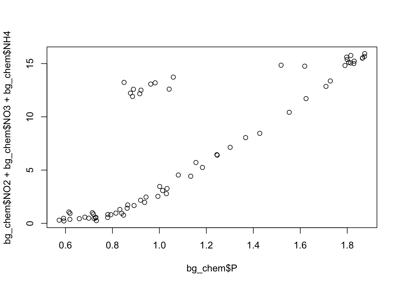
As our “analysis” we are going to calculate some very simple summary statistics and generate a single plot. In this dataset of oceanographic water samples, we will be examining the ratio of nitrogen to phosphate to see how closely the data match the Redfield ratio, which is the consistent 16:1 ratio of nitrogen to phosphorous atoms found in marine phytoplankton.
Under the appropriate bullet point in your analysis section, create a new R chunk, and use it to calculate the mean nitrate (NO3), nitrite (NO2), ammonium (NH4), and phosphorous (P) measured. Save these mean values as new variables with easily understandable names, and write a (brief) description of your operation using markdown above the chunk.
nitrate <- mean(bg_chem$NO3)
nitrite <- mean(bg_chem$NO2)
amm <- mean(bg_chem$NH4)
phos <- mean(bg_chem$P)
In another chunk, use those variables to calculate the nitrogen:phosphate ratio (Redfield ratio).
You can access this variable in your Markdown text by using R in-line in your text. The syntax to call R in-line (as opposed to as a chunk) is a single backtick `, the letter “r”, whatever your simple R command is - here we will use round(ratio) to print the calculated ratio, and a closing backtick `. So: ` 6 `. This allows us to access the value stored in this variable in our explanatory text without resorting to the evaluate-copy-paste method so commonly used for this type of task. The text as it looks in your RMrakdown will look like this:
The Redfield ratio for this dataset is approximately `r round(ratio)`.
And the rendered text like this:
The Redfield ratio for this dataset is approximately 6.
Finally, create a simple plot using base R that plots the ratio of the individual measurements, as opposed to looking at mean ratio.
Challenge
Decide whether or not you want the plotting code above to show up in your knitted document along with the plot, and implement your decision as a chunk option.
“Knit” your RMarkdown document (by pressing the Knit button) to observe the results.
Aside
How do I decide when to make a new chunk?
Like many of life’s great questions, there is no clear cut answer. My preference is to have one chunk per functional unit of analysis. This functional unit could be 50 lines of code or it could be 1 line, but typically it only does one “thing.” This could be reading in data, making a plot, or defining a function. It could also mean calculating a series of related summary statistics (as above). Ultimately the choice is one related to personal preference and style, but generally you should ensure that code is divided up such that it is easily explainable in a literate analysis as the code is run.
5.6.6 RMarkdown and environments
Let’s walk through an exercise with the document you built together to demonstrate how RMarkdown handles environments. We will be deliberately inducing some errors here for demonstration purposes.
First, follow these steps:
- Restart your R session (Session > Restart R)
- Run the last chunk in your Rmarkdown by pressing the play button on the chunk
Perhaps not surprisingly, we get an error:
Error in plot(bg_chem$P, bg_chem$NO2 + bg_chem$NO3 + bg_chem$NH4) :
  object 'bg_chem' not found
This is because we have not run the chunk of code that reads in the bg_chem data. The R part of Rmarkdown works just like a regular R script. You have to execute the code, and the order that you run it in matters. It is relatively easy to get mixed up in a large RMarkdown document - running chunks out of order, or forgetting to run chunks. To resolve this, follow the next step:
- Select from the “Run” menu (top right of Rmarkdown editor) “Restart R and run all chunks”
- Observe the
bg_chemvariable in your environment.
This is one of my favorite ways to reset and re-run my code when things seem to have gone sideways. This is great practice to do periodically since it helps ensure you are writing code that actually runs.
For the next demonstration:
- Restart your R session (Session > Restart R)
- Press Knit to run all of the code in your document
- Observe the state of your environment pane
Assuming your document knitted and produced an html page, your code ran. Yet the environment pane is empty. What happened?
The Knit button is rather special - it doesn’t just run all of the code in your document. It actually spins up a fresh R environment separate from the one you have been working in, runs all of the code in your document, generates the output, and then closes the environment. This is one of the best ways RMarkdown helps ensure you have built a reproducible workflow. If, while you were developing your code, you ran a line in the console as opposed to adding it to your RMarkdown document, the code you develop while working actively in your environment will still work. However, when you knit your document, the environment RStudio spins up doesn’t know anything about that working environment you were in. Thus, your code may error because it doesn’t have that extra piece of information. Commonly, library calls are the source of this kind of frustration when the author runs it in the console, but forgets to add it to the script.
To further clarify the point on environments, perform the following steps:
- Select from the “Run” menu (top right of Rmarkdown editor) “Run All”
- Observe all of the variables in your environment.
Aside
What about all my R scripts?
Some pieces of R code are better suited for R scripts than RMarkdown. A function you wrote yourself that you use in many different analyses is probably better to define in an R script than repeated across many RMarkdown documents. Some analyses have mundane or repetitive tasks that don’t need to be explained very much. For example, in the document shown in the beginning of this lesson, 15 different excel files needed to be reformatted in slightly different, mundane ways, like renaming columns and removing header text. Instead of including these tasks in the primary markdown, I instead chose to write one R script per file and stored them all in a directory. I took the contents of one script and included it in my literate analysis, using it as an example to explain what the scripts did, and then used the source function to run them all from within my RMarkdown.
So, just because you know RMarkdown now, doesn’t mean you won’t be using R scripts anymore. Both .R and .Rmd have their roles to play in analysis. With practice, it will become more clear what works well in RMarkdown, and what belongs in a regular R script.
5.6.7 Go Further
Create an RMarkdown document with some of your own data. If you don’t have a good dataset handy, use the example dataset here:
Your document might contain the following sections:
Introduction to your dataset
- Include an external link
Simple analysis
Presentation of a result
- A table
- An in-line R command
5.6.8 Resources
5.6.9 Troubleshooting
5.6.9.1 My RMarkdown won’t knit to PDF
If you get an error when trying to knit to PDF that says your computer doesn’t have a LaTeX installation, one of two things is likely happening:
- Your computer doesn’t have LaTeX installed
- You have an installation of LaTeX but RStudio cannot find it (it is not on the path)
If you already use LaTeX (like to write papers), you fall in the second category. Solving this requires directing RStudio to your installation - and isn’t covered here.
If you fall in the first category - you are sure you don’t have LaTeX installed - can use the R package tinytex to easily get an installation recognized by RStudio, as long as you have administrative rights to your computer.
To install tinytex run:
If you get an error that looks like destination /usr/local/bin not writable, you need to give yourself permission to write to this directory (again, only possible if you have administrative rights). To do this, run this command in the terminal:
sudo chown -R `whoami`:admin /usr/local/binand then try the above install instructions again. More information about tinytex can be found here
5.7 Version Control with git and GitHub
5.7.1 Learning Objectives
In this lesson, you will learn:
- Why git is useful for reproducible analysis
- How to use git to track changes to your work over time
- How to use GitHub to collaborate with others
- How to structure your commits so your changes are clear to others
- How to write effective commit messages
5.7.2 Introduction to git
Every file in the scientific process changes. Manuscripts are edited.
Figures get revised. Code gets fixed when problems are discovered. Data files
get combined together, then errors are fixed, and then they are split and
combined again. In the course of a single analysis, one can expect thousands of
changes to files. And yet, all we use to track this are simplistic filenames.
You might think there is a better way, and you’d be right: version control.
Version control systems help you track all of the changes to your files, without
the spaghetti mess that ensues from simple file renaming. In version control systems
like git, the system tracks not just the name of the file, but also its contents,
so that when contents change, it can tell you which pieces went where. It tracks
which version of a file a new version came from. So its easy to draw a graph
showing all of the versions of a file, like this one:
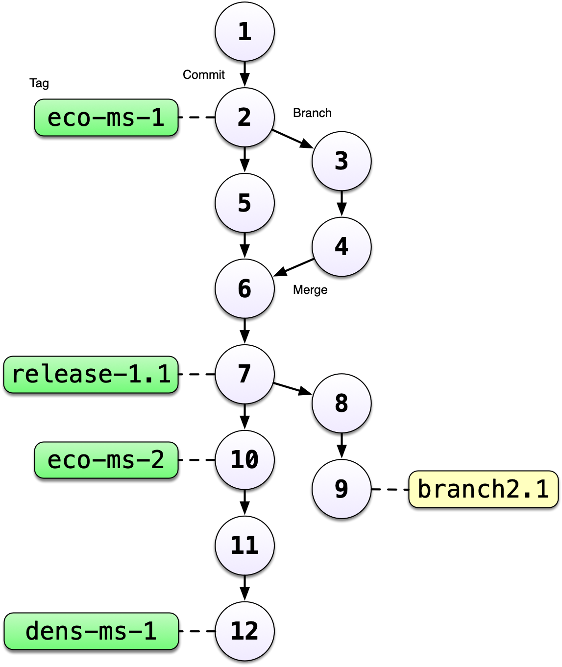
Version control systems assign an identifier to every version of every file, and
track their relationships. They also allow branches in those versions, and merging
those branches back into the main line of work. They also support having
multiple copies on multiple computers for backup, and for collaboration.
And finally, they let you tag particular versions, such that it is easy to return
to a set of files exactly as they were when you tagged them. For example, the
exact versions of data, code, and narrative that were used when a manuscript was originally
submitted might be eco-ms-1 in the graph above, and then when it was revised and resubmitted,
it was done with tag eco-ms-2. A different paper was started and submitted with tag dens-ms-1, showing that you can be working on multiple manuscripts with closely related but not identical sets of code and data being used for each, and keep track of it all.
Version control and Collaboration using Git and GitHub
First, just what are git and GitHub?
- git: version control software used to track files in a folder (a repository)
- git creates the versioned history of a repository
- GitHub: web site that allows users to store their git repositories and share them with others
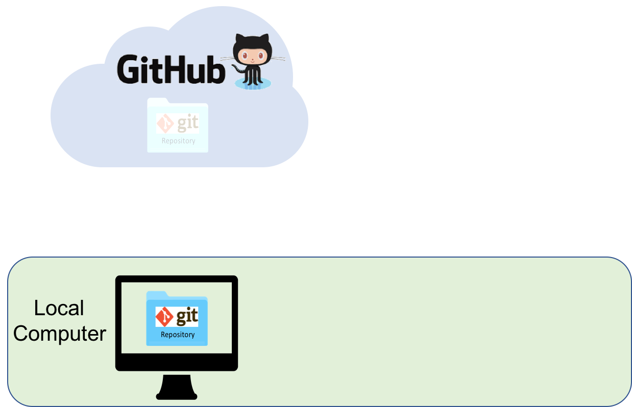
Let’s look at a GitHub repository
This screen shows the copy of a repository stored on GitHub, with its list of files, when the files and directories were last modified, and some information on who made the most recent changes.
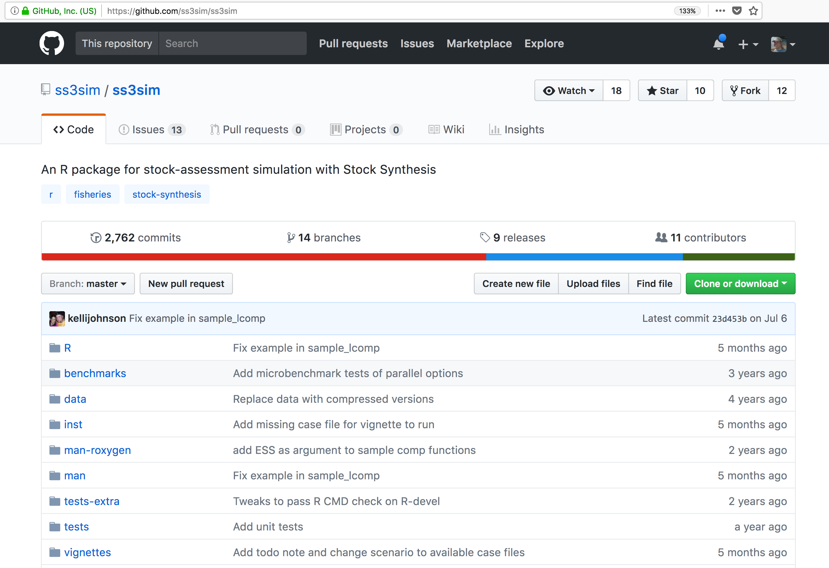 If we drill into the
“commits” for the repository, we can see the history of changes made to all of
the files. Looks like
If we drill into the
“commits” for the repository, we can see the history of changes made to all of
the files. Looks like kellijohnson and seananderson were fixing things in
June and July:
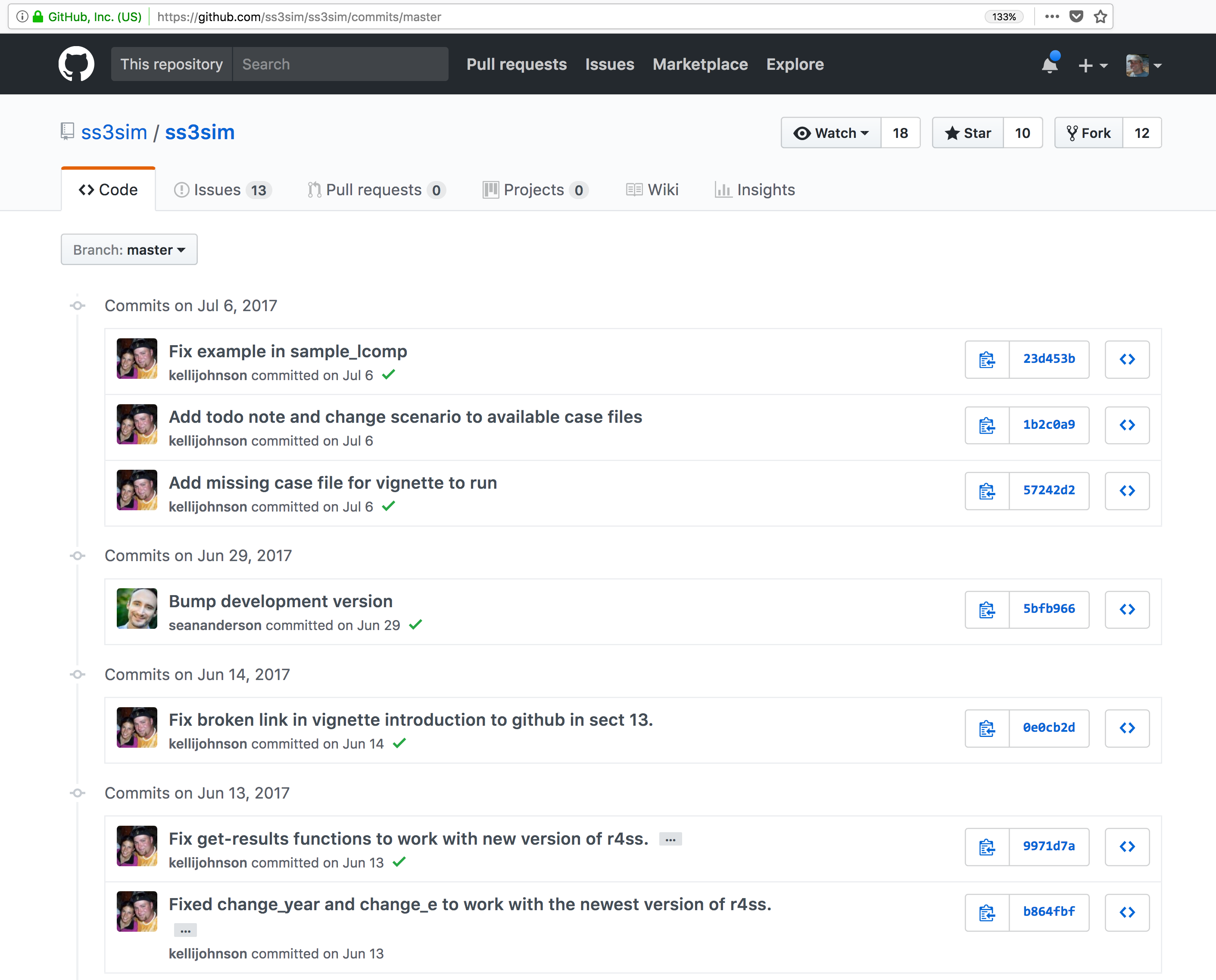
And finally, if we drill into the changes made on June 13, we can see exactly what was changed in each file:
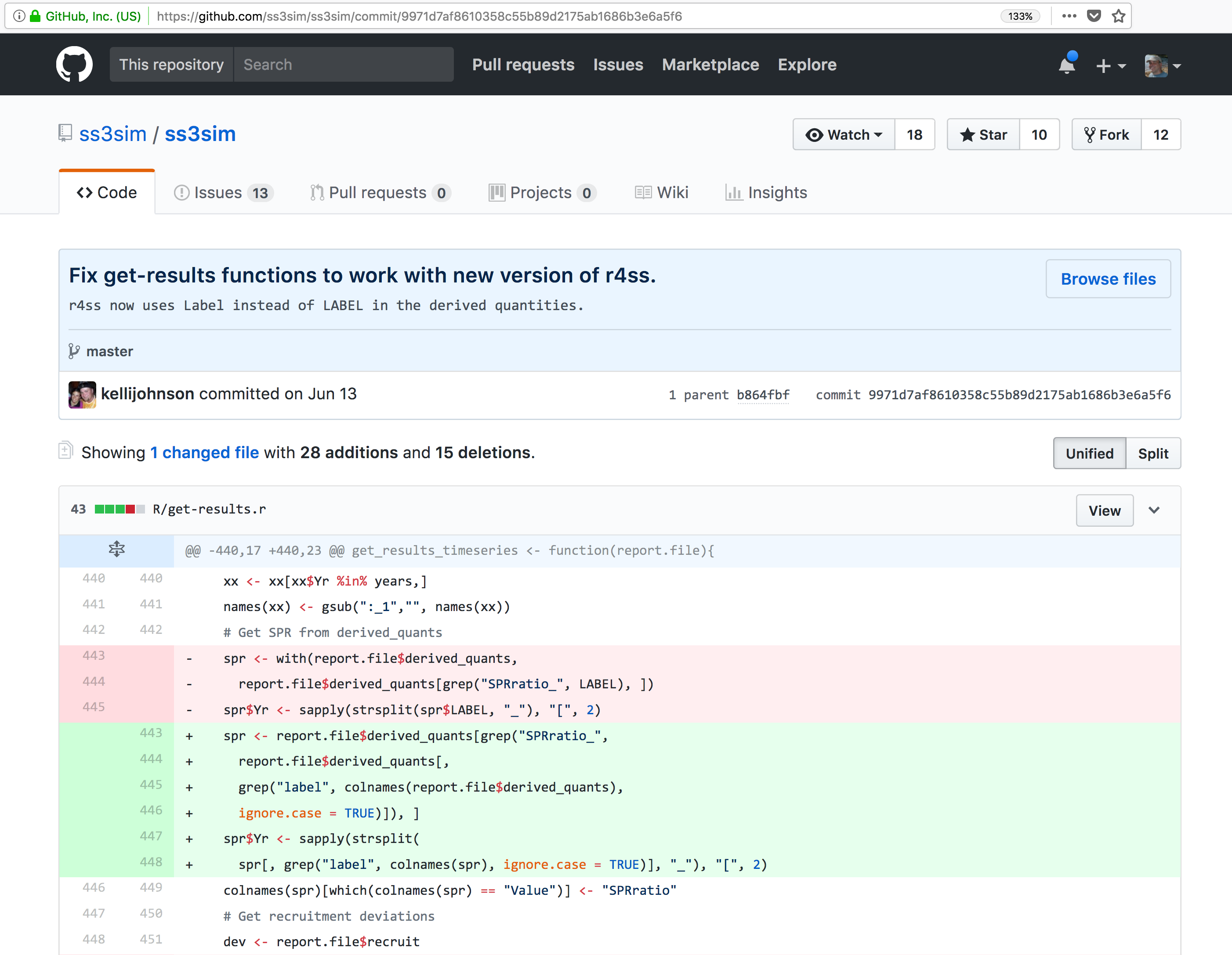 Tracking these changes, how they relate to released versions of software and files
is exactly what Git and GitHub are good for. And we will show how they can really
be effective for tracking versions of scientific code, figures, and manuscripts
to accomplish a reproducible workflow.
Tracking these changes, how they relate to released versions of software and files
is exactly what Git and GitHub are good for. And we will show how they can really
be effective for tracking versions of scientific code, figures, and manuscripts
to accomplish a reproducible workflow.
The Git lifecycle
As a git user, you’ll need to understand the basic concepts associated with versioned sets of changes, and how they are stored and moved across repositories. Any given git repository can be cloned so that it exist both locally, and remotely. But each of these cloned repositories is simply a copy of all of the files and change history for those files, stored in git’s particular format. For our purposes, we can consider a git repository just a folder with a bunch of additional version-related metadata.
In a local git-enabled folder, the folder contains a workspace containing the current version of all files in the repository. These working files are linked to a hidden folder containing the ‘Local repository’, which contains all of the other changes made to the files, along with the version metadata.
So, when working with files using git, you can use git commands to indicate specifically
which changes to the local working files should be staged for versioning
(using the git add command), and when to record those changes as a version in
the local repository (using the command git commit).
The remaining concepts are involved in synchronizing the changes in your local
repository with changes in a remote repository. The git push command is used to
send local changes up to a remote repository (possibly on GitHub), and the git pull
command is used to fetch changes from a remote repository and merge them into the
local repository.
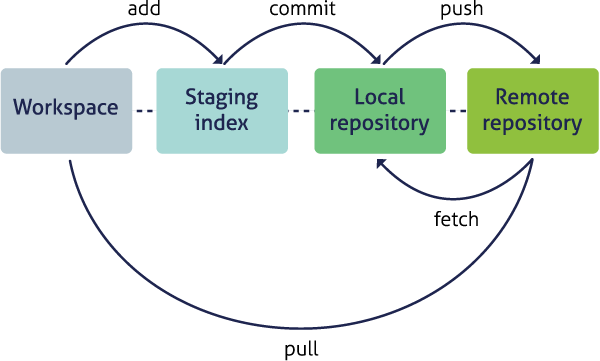
git clone: to copy a whole remote repository to localgit add(stage): notify git to track particular changesgit commit: store those changes as a versiongit pull: merge changes from a remote repository to our local repositorygit push: copy changes from our local repository to a remote repositorygit status: determine the state of all files in the local repositorygit log: print the history of changes in a repository
Those seven commands are the majority of what you need to successfully use git.
But this is all super abstract, so let’s explore with some real examples.
5.7.3 Create a remote repository on GitHub
Let’s start by creating a repository on GitHub, then we’ll edit some files.
Setup
- Log into GitHub
- Click the New repository button
- Name it
training-test - Create a README.md
- Set the LICENSE to Apache 2.0
- Add a .gitignore file for
R
If you were successful, it should look something like this:
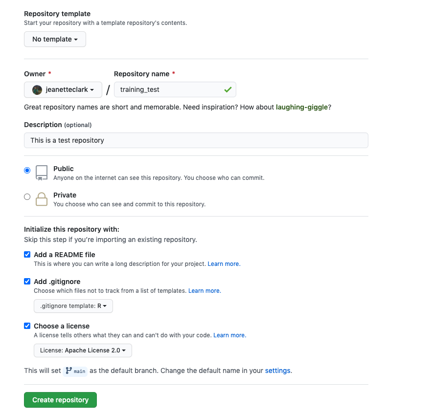
You’ve now created your first repository! It has a couple of files that GitHub created for you, like the README.md file, and the LICENSE file, and the .gitignore file.
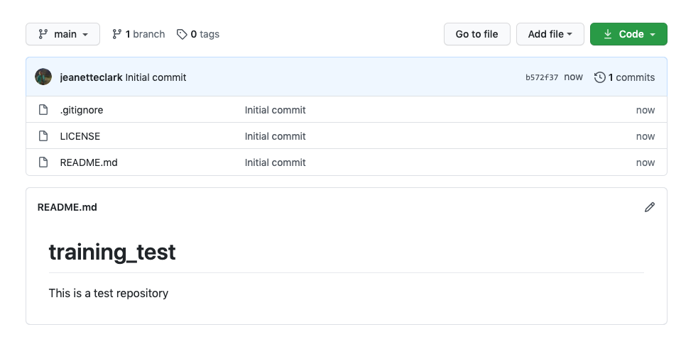
For simple changes to text files, you can make edits right in the GitHub web interface.
Challenge
Navigate to the README.md file in the file listing, and edit it by clicking on the pencil icon.
This is a regular Markdown file, so you can just add markdown text. When done, add a commit message, and
hit the Commit changes button.
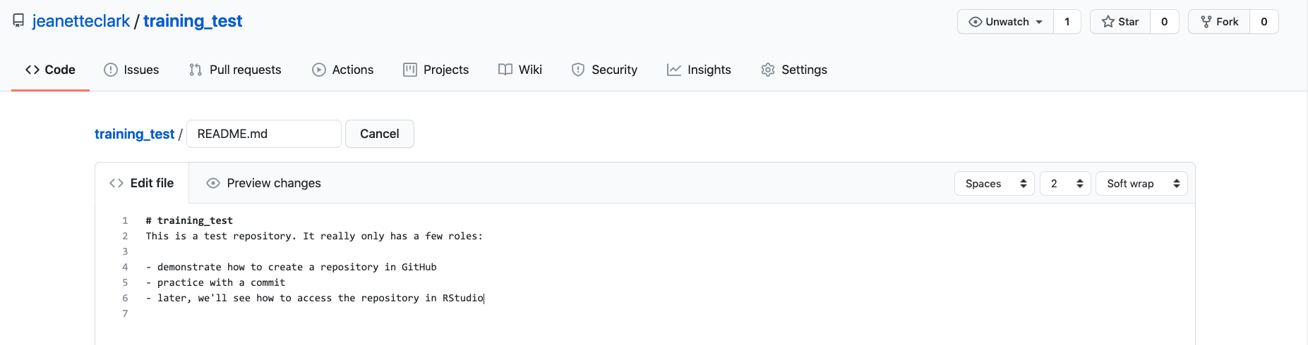
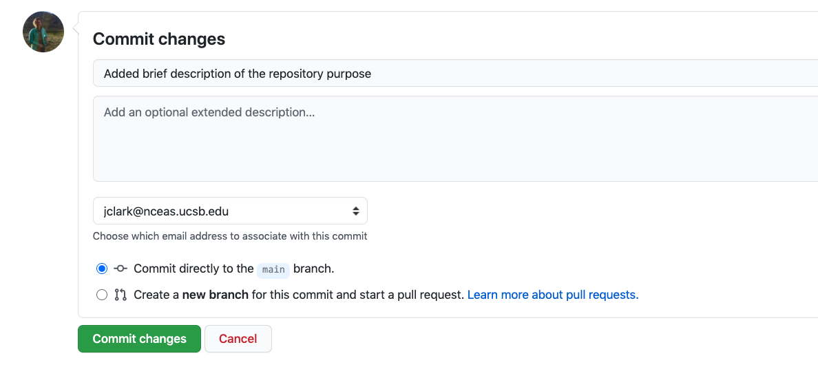
Congratulations, you’ve now authored your first versioned commit. If you navigate back to the GitHub page for the repository, you’ll see your commit listed there, as well as the rendered README.md file.
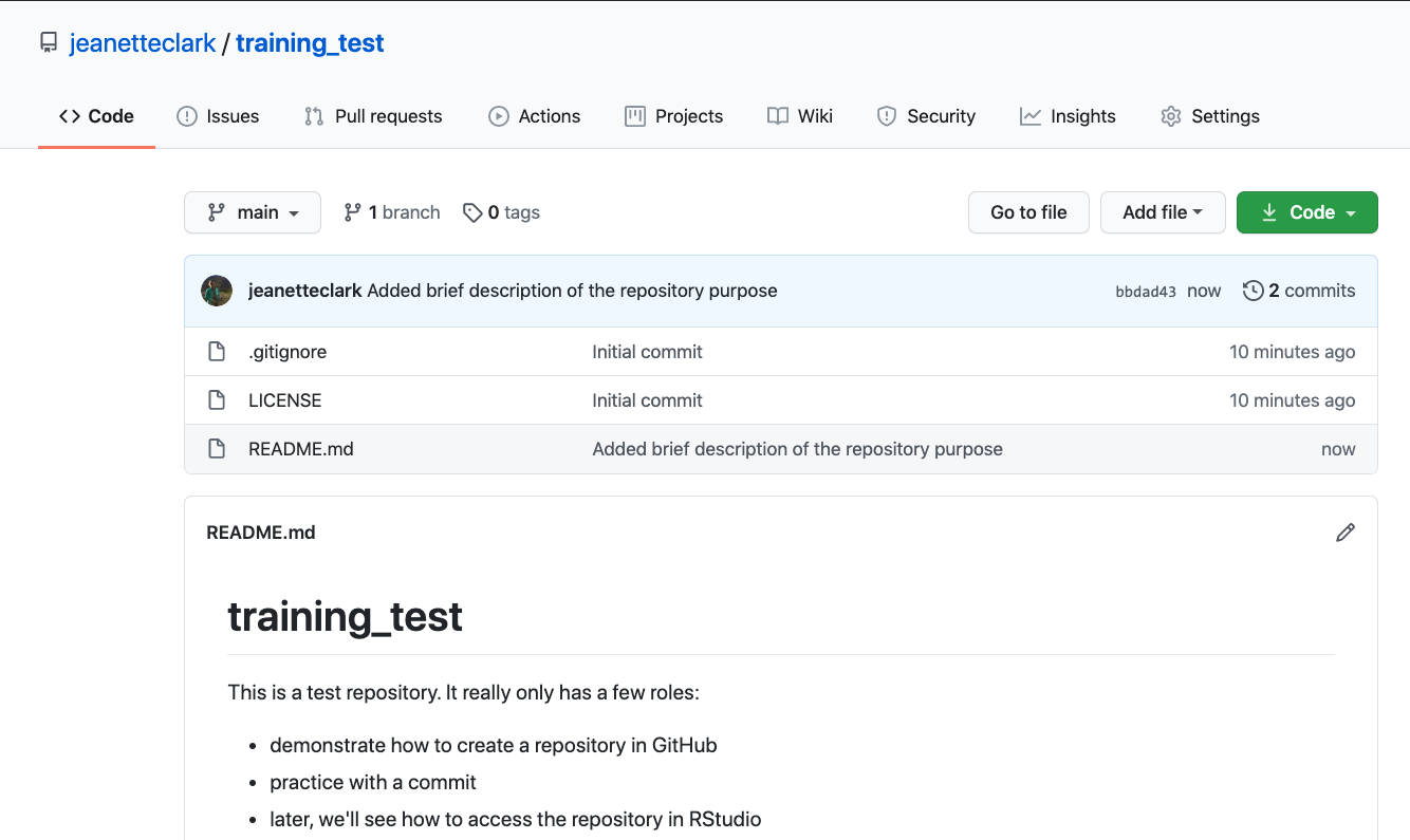
Let’s point out a few things about this window. It represents a view of the repository that you created, showing all of the files in the repository so far. For each file, it shows when the file was last modified, and the commit message that was used to last change each file. This is why it is important to write good, descriptive commit messages. In addition, the blue header above the file listing shows the most recent commit, along with its commit message, and its SHA identifier. That SHA identifier is the key to this set of versioned changes. If you click on the SHA identifier (810f314), it will display the set of changes made in that particular commit.
In the next section we’ll use the GitHub URL for the GitHub repository you created
to clone the repository onto your local machine so that you can edit the files
in RStudio. To do so, start by copying the GitHub URL, which represents the repository
location:
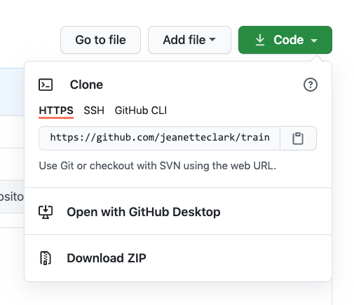
5.7.4 Working locally with Git via RStudio
For convenience, it would be nice to be able to edit the files locally on our
computer using RStudio rather than working on the GitHub website. We can do this
by using the clone command to copy the repository from GitHub to our local computer,
which then allows us to push changes up to GitHub and pull down any changes that
have occurred.
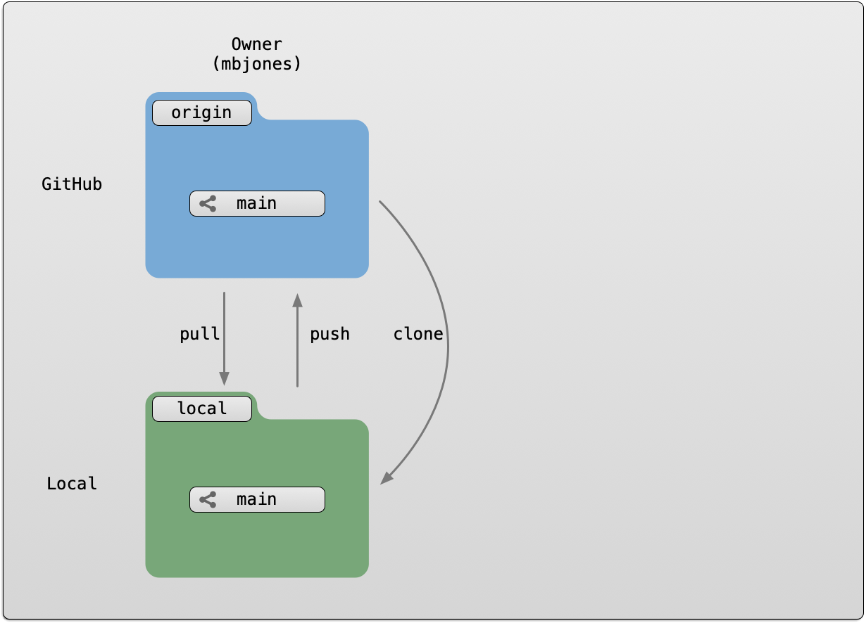
We refer to the remote copy of the repository that is on GitHub as the origin
repository (the one that we cloned from), and the copy on our local computer as
the local copy.
RStudio knows how to work with files under version control with Git, but only if you are working within an RStudio project folder. In this next section, we will clone the repository that you created on GitHub into a local repository as an RStudio project. Here’s what we’re going to do:
- Create the new project
- Inspect the Git tab and version history
- Commit a change to the README.md file
- Commit the changes that RStudio made
- Inspect the version history
- Add and commit an Rmd file
- Push these changes to GitHub
- View the change history on GitHub
Setup
In the File menu, select “New Project.” In the dialog that pops up, select the “Version Control” option, and paste the GitHub URL that you copied into the field for the remote repository Repository URL. While you can name the local copy of the repository anything, it’s typical to use the same name as the GitHub repository to maintain the correspondence.
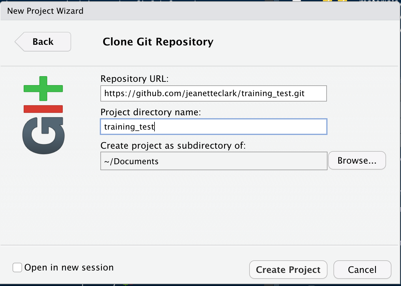
Once you hit `Create Project, a new RStudio window will open with all of the files from the remote repository copied locally. Depending on how your version of RStudio is configured, the location and size of the panes may differ, but they should all be present, including a Git tab and the normal Files tab listing the files that had been created in the remote repository.
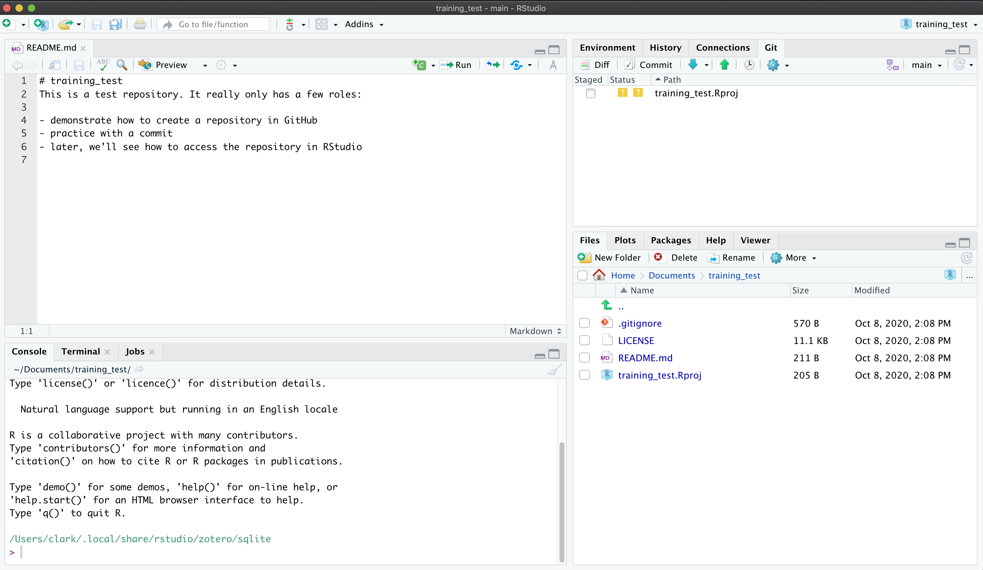
You’ll note that there is one new file training-test.Rproj, and three files that we
created earlier on GitHub (.gitignore, LICENSE, and README.md).
In the Git tab, you’ll note that two files are listed. This is the status pane
that shows the current modification status of all of the files in the repository.
In this case, the .gitignore file is listed as M for Modified, and training-test.Rproj
is listed with a ? ? to indicate that the file is untracked. This means that
git has not stored any versions of this file, and knows nothing about the file.
As you make version control decisions in RStudio, these icons will change to reflect
the current version status of each of the files.
Inspect the history. For now, let’s click on the History button in the Git tab, which will show the log of changes that occurred, and will be identical to what we viewed on GitHub. By clicking on each row of the history, you can see exactly what was added and changed in each of the two commits in this repository.
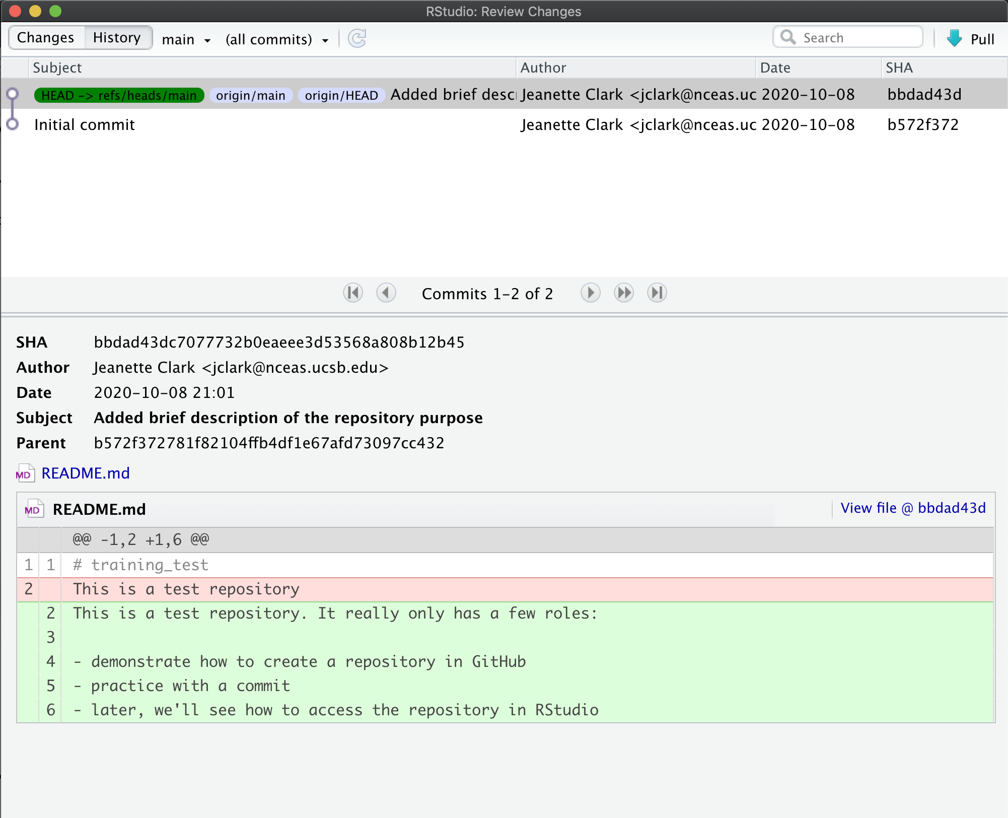
Challenge
Commit a README.md change. Next let’s make a change to the README.md file, this time from RStudio.
Add a new section to your markdown using a header, and under it include a list three advantages to using git.
Once you save, you’ll immediately see the README.md file show up in the Git tab, marked as a modification. You can select the file in the Git tab, and click Diff to see the differences that you saved (but which are not yet committed to your local repository).
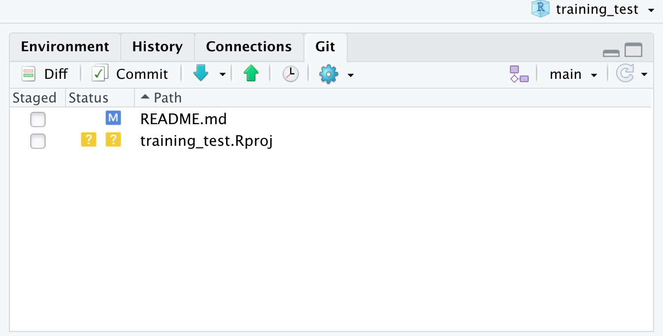
And here’s what the newly made changes look like compared to the original file. New lines are highlighted in green, while removed lines are in red.
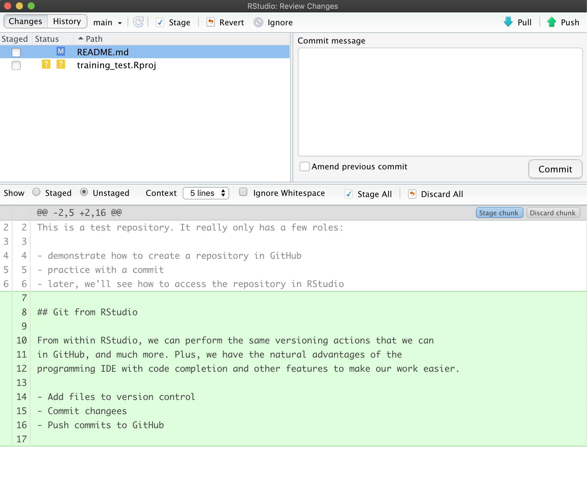 Commit the RStudio changes.
To commit the changes you made to the README.md file, check the Staged checkbox next to the file (which tells Git which changes you want included in the commit), then provide a descriptive Commit message, and then click Commit.
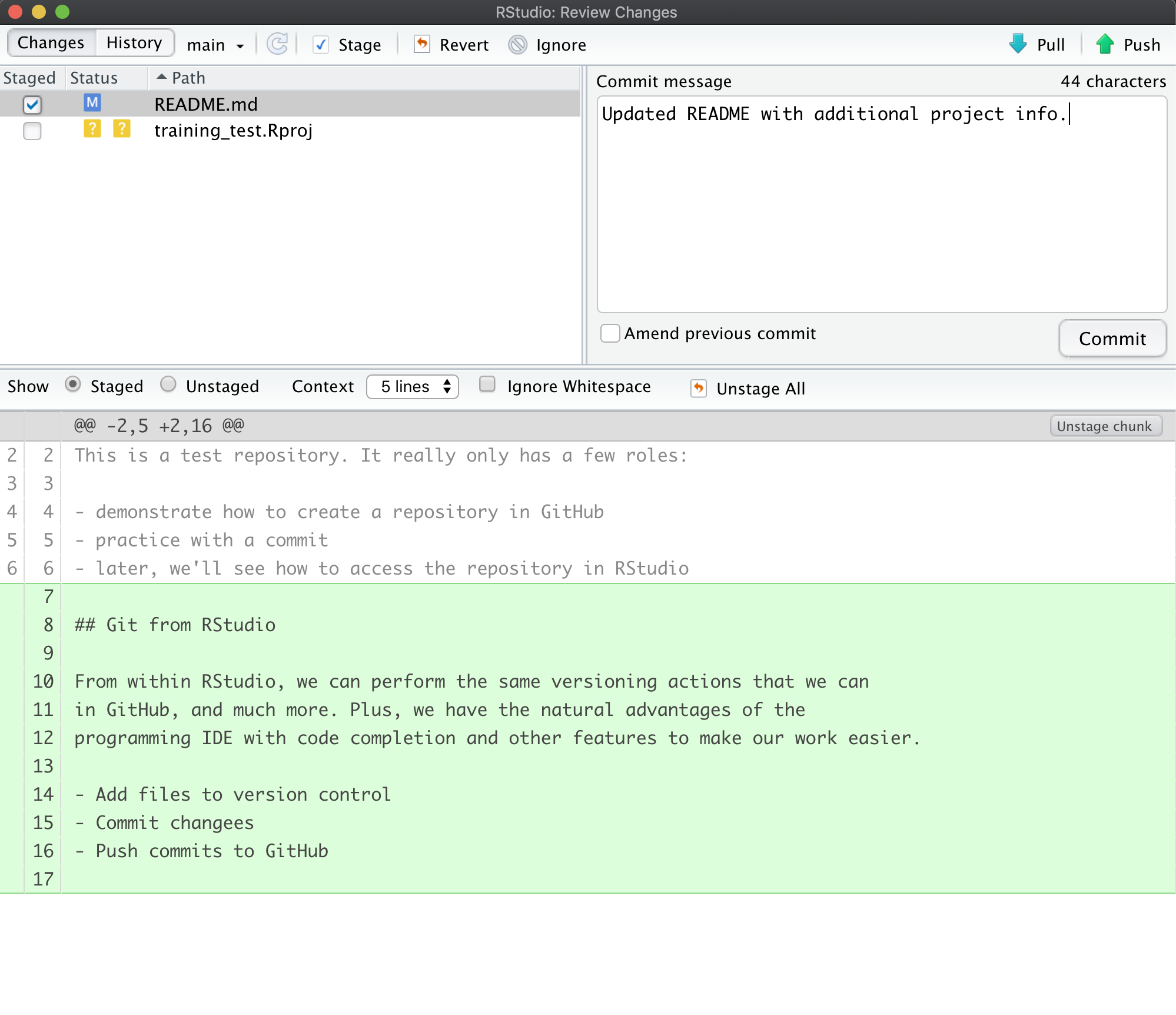
Note that some of the changes in the repository, namely training-test.Rproj are still listed as having not been committed. This means
there are still pending changes to the repository. You can also see the note
that says:
Your branch is ahead of ‘origin/main’ by 1 commit.
This means that we have committed 1 change in the local repository, but that
commit has not yet been pushed up to the origin repository, where origin
is the typical name for our remote repository on GitHub. So, let’s commit the
remaining project files by staging them and adding a commit message.
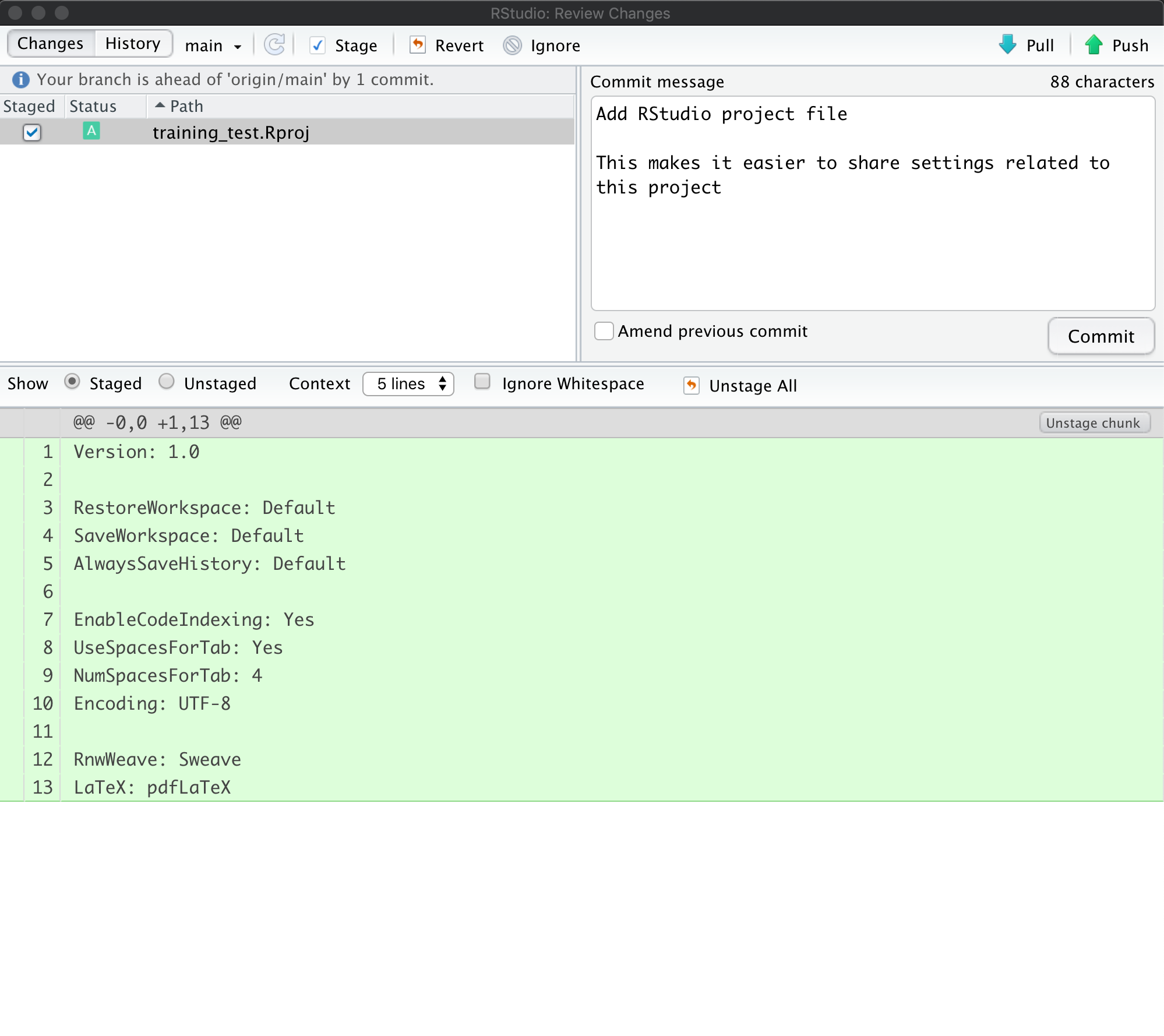
When finished, you’ll see that no changes remain in the Git tab, and the repository is clean.
Inspect the history. Note that the message now says:
Your branch is ahead of ‘origin/main’ by 2 commits.
These 2 commits are the two we just made, and have not yet been pushed to GitHub. By clicking on the History button, we can see that there are now a total of four commits in the local repository (while there had only been two on GitHub).
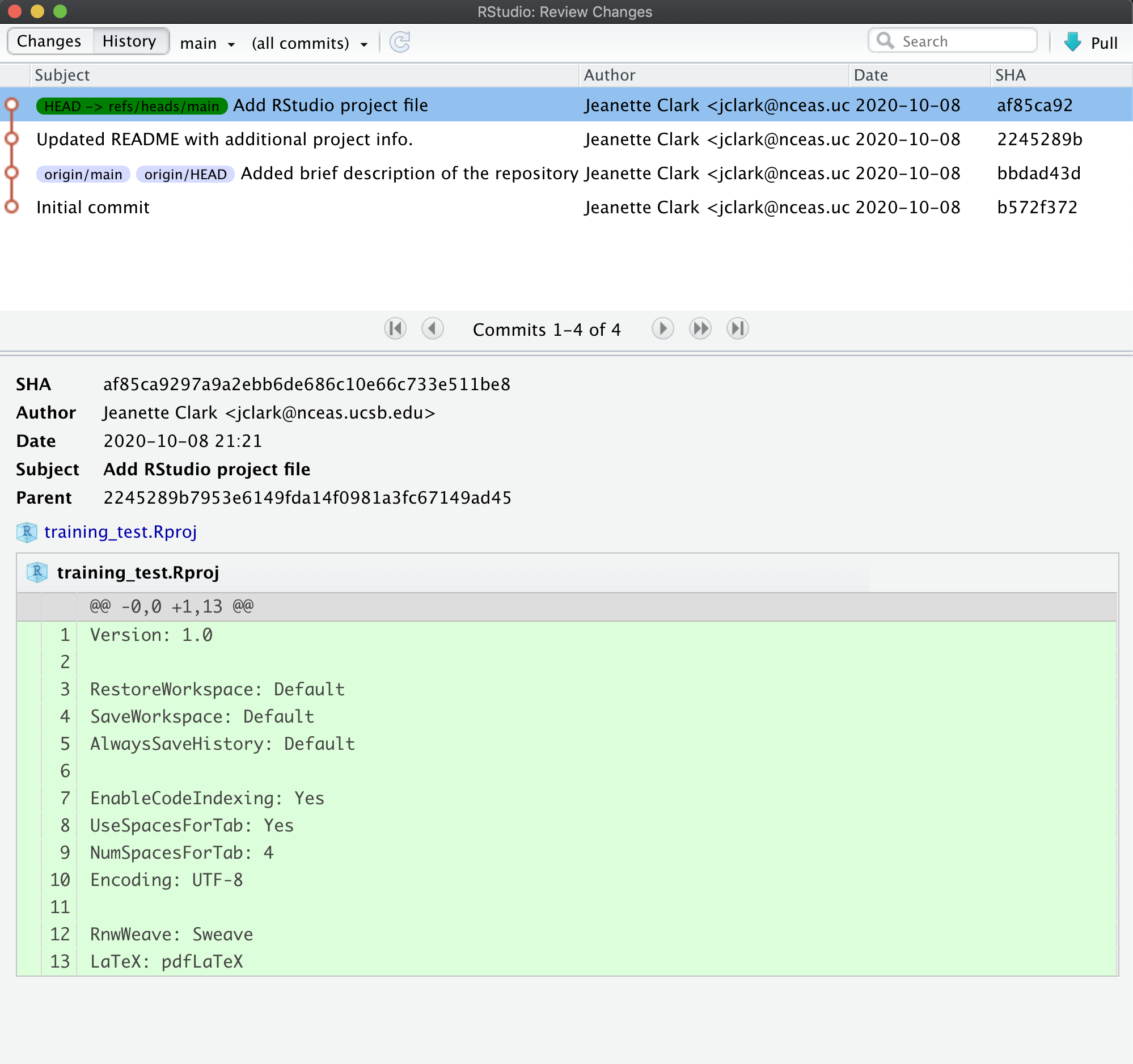
Push these changes to GitHub. Now that everything has been changed as desired locally, you can push the changes to GitHub using the Push button. This will prompt you for your GitHub username and password, and upload the changes, leaving your repository in a totally clean and synchronized state. When finished, looking at the history shows all four commits, including the two that were done on GitHub and the two that were done locally on RStudio.
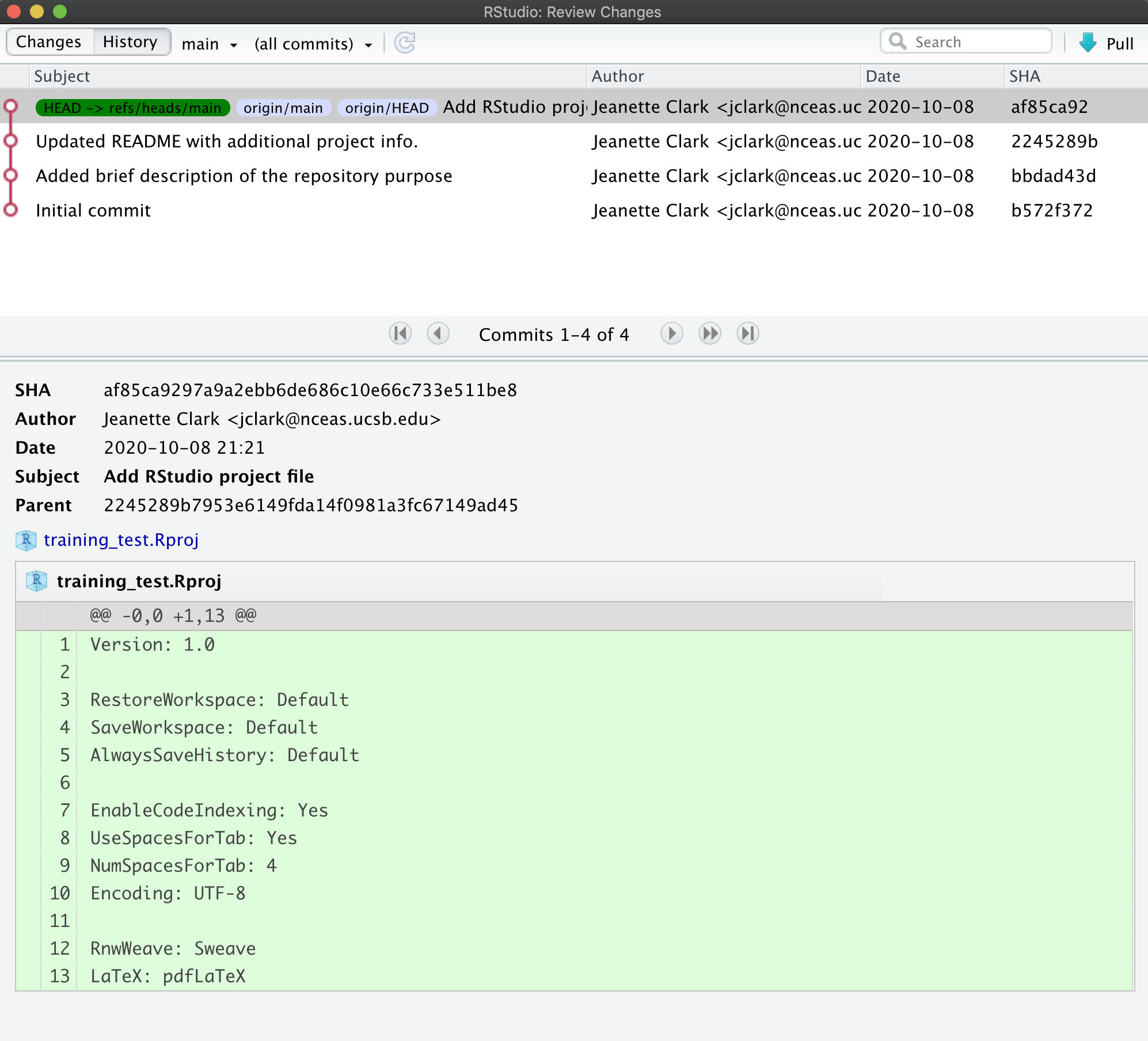
And note that the labels indicate that both the local repository (HEAD) and the
remote repository (origin/HEAD) are pointing at the same version in the history.
So, if we go look at the commit history on GitHub, all the commits will be shown
there as well.
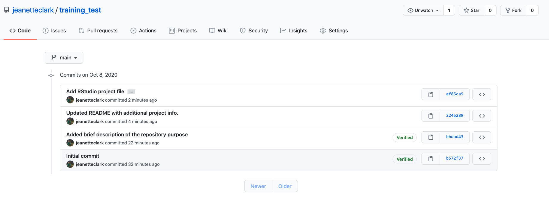
Aside
What should I write in my commit message?
Clearly, good documentation of what you’ve done is critical to making the version history of your repository meaningful and helpful. Its tempting to skip the commit message altogether, or to add some stock blurb like ‘Updates’. It’s better to use messages that will be helpful to your future self in deducing not just what you did, but why you did it. Also, commit messaged are best understood if they follow the active verb convention. For example, you can see that my commit messages all started with a past tense verb, and then explained what was changed.
While some of the changes we illustrated here were simple and so easily explained in a short phrase, for more complex changes, its best to provide a more complete message. The convention, however, is to always have a short, terse first sentence, followed by a more verbose explanation of the details and rationale for the change. This keeps the high level details readable in the version log. I can’t count the number of times I’ve looked at the commit log from 2, 3, or 10 years prior and been so grateful for diligence of my past self and collaborators.
Collaboration and conflict free workflows
Up to now, we have been focused on using Git and GitHub for yourself, which is a great use. But equally powerful is to share a GitHub repository with other researchers so that you can work on code, analyses, and models together. When working together, you will need to pay careful attention to the state of the remote repository to avoid and handle merge conflicts. A merge conflict occurs when two collaborators make two separate commits that change the same lines of the same file. When this happens, git can’t merge the changes together automatically, and will give you back an error asking you to resolve the conflict. Don’t be afraid of merge conflicts, they are pretty easy to handle. and there are some great guides.
That said, its truly painless if you can avoid merge conflicts in the first place. You can minimize conflicts by:
- Ensure that you pull down changes just before you commit
- Ensures that you have the most recent changes
- But you may have to fix your code if conflict would have occurred
- Coordinate with your collaborators on who is touching which files
- You still need to communicate to collaborate
5.7.5 Setting up git on an existing project
Now you have two projects set up in your RStudio environment, training_{USERNAME} and training_test. We set you up with the training_test project since we think it is an easy way to introduce you to git, but more commonly researchers will have an existing directory of code that they then want to make a git repository out of. For the last exercise of this session, we will do this with your training_{USERNAME} project.
First, switch to your training_{USERNAME} project using the RStudio project switcher. The project switcher is in the upper right corner of your RStudio pane. Click the dropdown next to your project name (training_test), and then select the training_{USERNAME} project from the “recent projects” list.
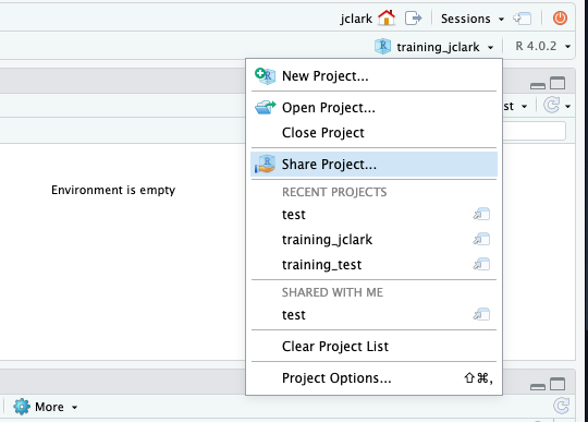
Next, from the Tools menu, select “Project Options.” In the dialog that pops up, select “Git/SVN” from the menu on the left. In the dropdown at the top of this page, select “Git” and click “Yes” in the confirmation box. Click “Yes” again to restart RStudio.
When RStudio restarts, you should have a git tab, with two untracked files (.gitignore and training_{USERNAME}.Rproj).
Challenge
Add and commit these two files to your git repository
Now we have your local repository all set up. You can make as many commits as you want on this repository, and it will likely still be helpful to you, but the power in git and GitHub is really in collaboration. As discussed, GitHub facilitates this, so let’s get this repository on GitHub.
Go back to GitHub, and click on the “New Repository” button.
In the repository name field, enter the same name as your RProject. So for me, this would be training_jclark. Add a description, keep the repository public, and, most importantly:
DO NOT INITIALIZE THE REPOSITORY WITH ANY FILES.
We already have the repository set up locally so we don’t need to do this. Initializing the repository will only cause merge issues.
Here is what your page should look like:
![]()
Once your page looks like that, click the “create repository” button.
This will open your empty repository with a page that conveniently gives you exactly the instructions you need. In our case, we are “pushing an existing repository from the command line.”
![]()
Click the clipboard icon to copy the code for the middle option of the three on this page. It should have three lines and look like this:
git remote add origin https://github.com/jeanetteclark/training_jclark.git
git branch -M main
git push -u origin main
Back in RStudio, open the terminal by clicking the tab labeled as such next to the console tab. The prompt should look something like this:
jclark@included-crab:~/training_jclark$In the prompt, paste the code that you copied from the GitHub page and press return. You will be prompted to type your GitHub username and password.
The code that you copied and pasted did three things:
- added the GitHub repository as the remote repository
- renamed the default branch to
main - pushed the
mainbranch to the remote GitHub repository
If you go back to your browser and refresh your GitHub repository page, you should now see your files appear.
Challenge
On your repository page, GitHub has a button that will help you add a readme file. Click the “Add a README” button and use markdown syntax to create a simple readme. Commit the changes to your repository.
Go to your local repository (in RStudio) and pull the changes you made.
5.7.6 Go Further
There’s a lot we haven’t covered in this brief tutorial. There are some great and much longer tutorials that cover advanced topics, such as:
Using git on the command line
Resolving conflicts
Branching and merging
Pull requests versus direct contributions for collaboration
Using .gitignore to protect sensitive data
GitHub Issues and why they are useful
and much, much more
Try Git is a great interactive tutorial
Software Carpentry Version Control with Git
Codecademy Learn Git (some paid)
5.8 Git Collaboration and Conflict Management
5.8.1 Learning Objectives
In this lesson, you will learn:
- How to use Git and GitHub to collaborate with colleagues on code
- What typically causes conflicts when collaborating
- Workflows to avoid conflicts
- How to resolve a conflict
5.8.2 Introduction
Git is a great tool for working on your own, but even better for working with friends and colleagues. Git allows you to work with confidence on your own local copy of files with the confidence that you will be able to successfully synchronize your changes with the changes made by others.
The simplest way to collaborate with Git is to use a shared repository on a hosting service such as GitHub, and use this shared repository as the mechanism to move changes from one collaborator to another. While there are other more advanced ways to sync git repositories, this “hub and spoke” model works really well due to its simplicity.
In this model, the collaborator will clone a copy of the owner’s repository from
GitHub, and the owner will grant them collaborator status, enabling the collaborator
to directly pull and push from the owner’s GitHub repository.
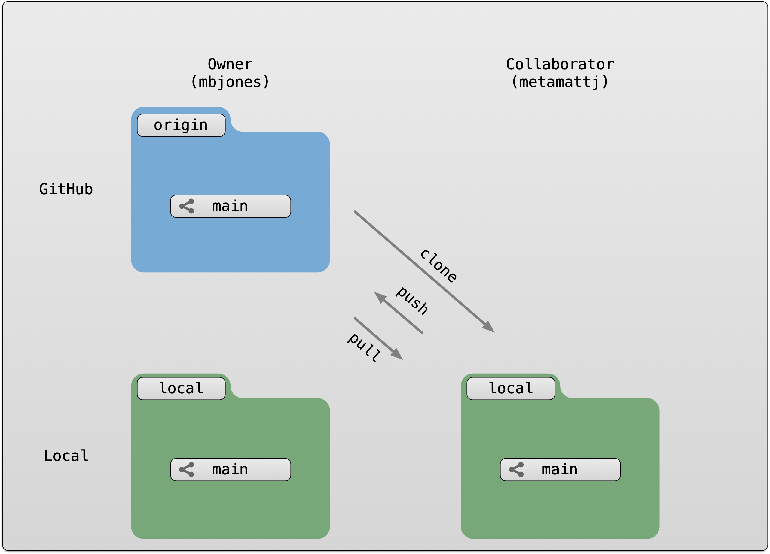
5.8.3 Collaborating with a trusted colleague without conflicts
We start by enabling collaboration with a trusted colleague. We will designate the Owner as the person who owns the shared repository, and the Collaborator as the person that they wish to grant the ability to make changes to their repository. We start by giving that person access to our GitHub repository.
Setup
- Work with a fellow postdoc or colleague, and choose one person as the
Ownerand one as theCollaborator - Log into GitHub as the `Owner
- Navigate to the
Owner’s training repository (e.g.,training_jones)
Then, have the Owner visit their training repository created earlier, and visit the Settings page, and select the Manage access screen, and add the username of your Collaborator in the box.
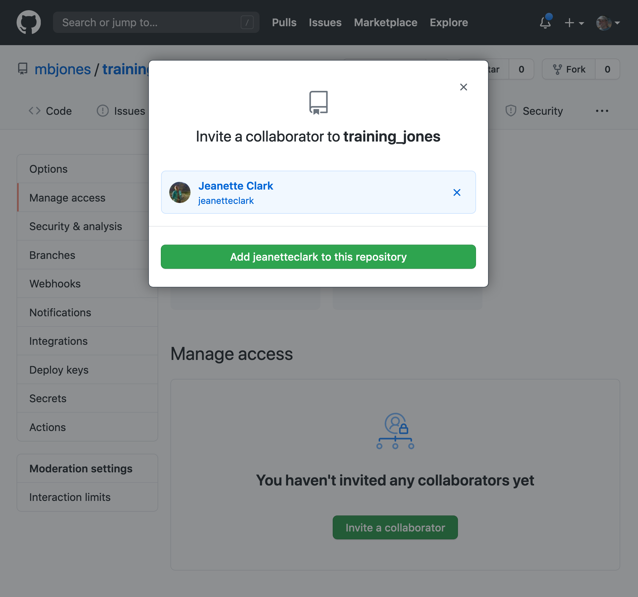
Once the collaborator has been added, they should check their email for an invitation from GitHub, and click on the acceptance link, which will enable them to collaborate on the repository.
We will start by having the collaborator make some changes and share those with the Owner without generating any conflicts, In an ideal world, this would be the normal workflow. Here are the typical steps.
5.8.3.1 Step 1: Collaborator clone
To be able to contribute to a repository, the collaborator must clone the repository from the Owner’s github account. To do this, the Collaborator should visit the github page for the Owner’s repository, and then copy the clone URL. In R Studio, the Collaborator will create a new project from version control by pasting this clone URL into the appropriate dialog (see the earlier chapter introducing GitHub).
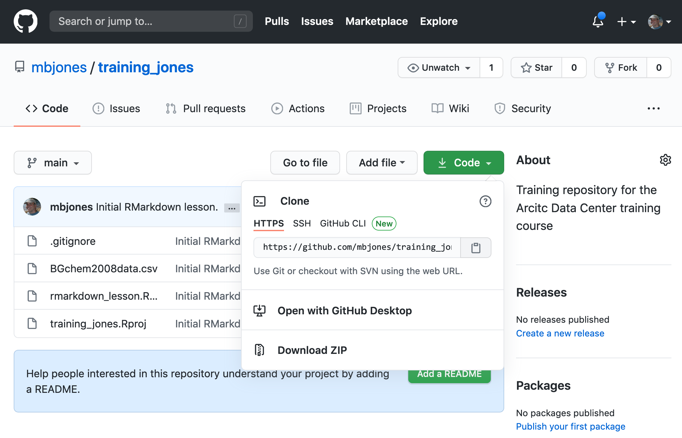
5.8.3.2 Step 2: Collaborator Edits
With a clone copied locally, the Collaborator can now make changes to the
index.Rmd file in the repository, adding a line or statment somewhere noticeable
near the top. Save your changes.
5.8.3.3 Step 3: Collaborator commit and push
To sync changes, the collaborator will need to add, commit, and
push their changes to the Owner’s repository. But before doing so, its good practice
to pull immediately before committing to ensure you have the most recent changes
from the owner. So, in R Studio’s Git tab, first click the “Diff” button to
open the git window, and then press the green “Pull” down arrow button. This will
fetch any recent changes from the origin repository and merge them. Next, add
the changed index.Rmd file to be committed by cicking the checkbox next to it,
type in a commit message, and click ‘Commit.’ Once that finishes, then the collaborator can
immediately click ‘Push’ to send the commits to the Owner’s GitHub repository.
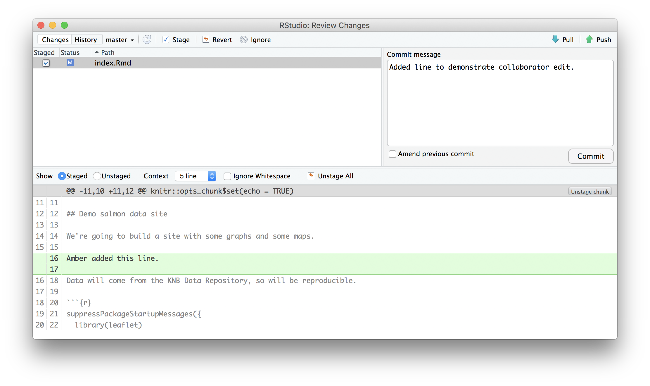
5.8.3.4 Step 4: Owner pull
Now, the owner can open their local working copy of the code
in RStudio, and pull those changes down to their local copy.
Congrats, the owner now has your changes!
5.8.3.5 Step 5: Owner edits, commit, and push
Next, the owner should do the same. Make changes to
a file in the repository, save it, pull to make sure no new changes have been made
while editing, and then add, commit, and push the Owner changes to GitHub.
5.8.3.6 Step 6: Collaborator pull
The collaborator can now pull down those owner changes,
and all copies are once again fully synced. And you’re off to collaborating.
Challenge
Try the same steps with your partner. Start by designating one person as the Owner and one as the Collborator, and then repeat the steps described above:
- Step 0: Setup permissions for your collaborator
- Step 1: Collaborator clones the Owner repository
- Step 2: Collaborator Edits the README file
- Step 3: Collaborator commits and pushes the file to GitHub
- Step 4: Owner pulls the changes that the Collaborator made
- Step 5: Owner edits, commits, and pushes some new changes
- Step 6: Collaborator pulls the owners changes from GitHub
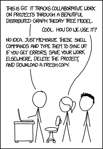
5.8.4 Merge conflicts
So things can go wrong, which usually starts with a merge conflict, due to both collaborators making incompatible changes to a file. While the error messages from merge conflicts can be daunting, getting things back to a normal state can be straightforward once you’ve got an idea where the problem lies.
A merge conflict occurs when both the owner and collaborator change the same lines in the same file without first pulling the changes that the other has made. This is most easily avoided by good communication about who is working on various sections of each file, and trying to avoid overlaps. But sometimes it happens, and git is there to warn you about potential problems. And git will not allow you to overwrite one person’s changes to a file with another’s changes to the same file if they were based on the same version.
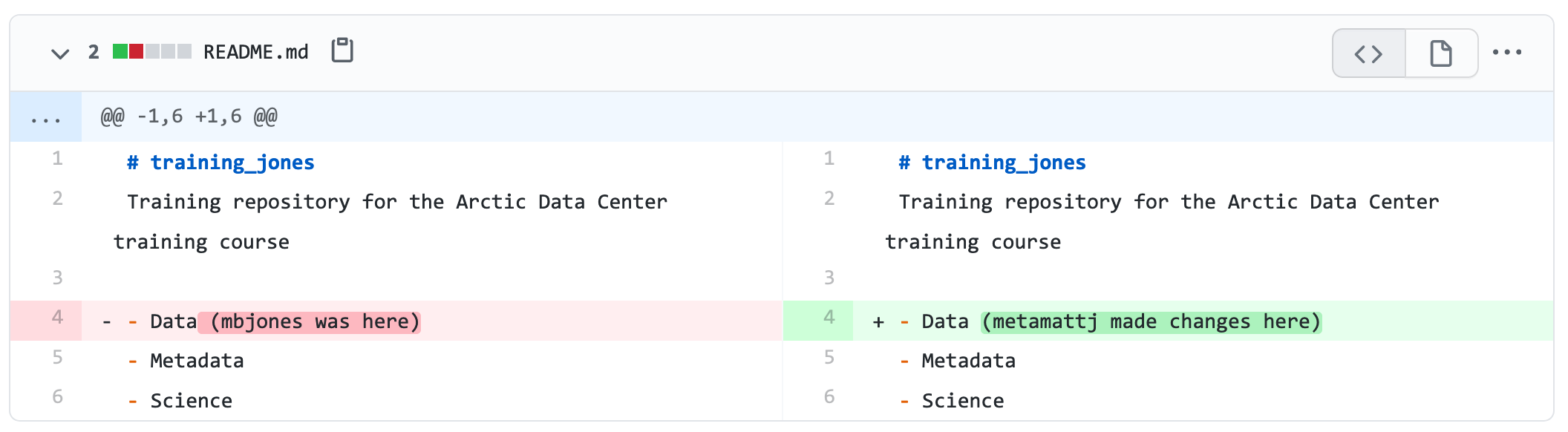
The main problem with merge conflicts is that, when the Owner and Collaborator both make changes to the same line of a file, git doesn’t know whose changes take precedence. You have to tell git whose changes to use for that line.
5.8.5 How to resolve a conflict
Abort, abort, abort…
Sometimes you just made a mistake. When you get a merge conflict, the repository is placed in a ‘Merging’ state until you resolve it. There’s a commandline command to abort doing the merge altogether:
git merge --abortOf course, after doing that you stull haven’t synced with your collaborator’s changes, so things are still unresolved. But at least your repository is now usable on your local machine.
Checkout
The simplest way to resolve a conflict, given that you know whose version of the
file you want to keep, is to use the commandline git program to tell git to
use either your changes (the person doing the merge), or their changes (the other collaborator).
- keep your collaborators file:
git checkout --theirs conflicted_file.Rmd - keep your own file:
git checkout --ours conflicted_file.Rmd
Once you have run that command, then run add, commit, and push the changes as normal.
Pull and edit the file
But that requires the commandline. If you want to resolve from RStudio, or if
you want to pick and choose some of your changes and some of your collaborator’s,
then instead you can manually edit and fix the file. When you pulled the file
with a conflict, git notices that there is a conflict and modifies the file to show
both your own changes and your collaborator’s changes in the file. It also shows the
file in the Git tab with an orange U icon, which indicates that the file is Unmerged,
and therefore awaiting you help to resolve the conflict. It delimits
these blocks with a series of less than and greater than signs, so they are easy to find:
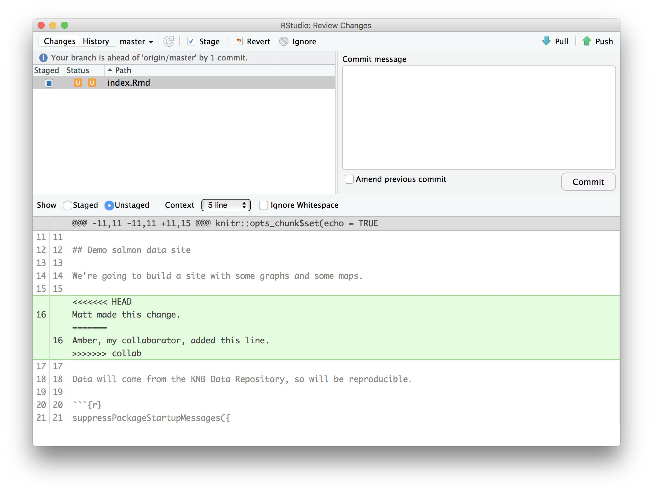
To resolve the conficts, simply find all of these blocks, and edit them so that
the file looks how you want (either pick your lines, your collaborators lines,
some combination, or something altogether new), and save. Be sure you removed the
delimiter lines that started with <<<<<<<, =======, and >>>>>>>.
Once you have made those changes, you simply add, commit, and push the files to resolve the conflict.
5.8.5.1 Producing and resolving merge conflicts
To illustrate this process, we’re going to carefully create a merge conflict step by step, show how to resolve it, and show how to see the results of the successful merge after it is complete. First, we will walk through the exercise to demonstrate the issues.
5.8.5.1.1 Owner and collaborator ensure all changes are updated
First, start the exercise by ensuring that both the Owner and Collaborator have all
of the changes synced to their local copies of the Owner’s repositoriy in RStudio.
This includes doing a git pull to ensure that you have all changes local, and
make sure that the Git tab in RStudio doesn’t show any changes needing to be committed.
5.8.5.1.2 Owner makes a change and commits
From that clean slate, the Owner first modifies and commits a small change inlcuding their name on a specific line of the README.md file (we will change line 4). Work to only change that one line, and add your username to the line in some form and commit the changes (but DO NOT push). We are now in the situation where the owner has unpushed changes that the collaborator can not yet see.
5.8.5.1.3 Collaborator makes a change and commits on the same line
Now the collaborator also makes changes to the same (line 4) of the README.md file in their RStudio copy of the project, adding their name to the line. They then commit. At this point, both the owner and collaborator have committed changes based on their shared version of the README.md file, but neither has tried to share their changes via GitHub.
5.8.5.1.4 Collaborator pushes the file to GitHub
Sharing starts when the Collaborator pushes their changes to the GitHub repo, which updates GitHub to their version of the file. The owner is now one revision behind, but doesn’t yet know it.
5.8.5.1.5 Owner pushes their changes and gets an error
At this point, the owner tries to push their change to the repository, which triggers an error from GitHub. While the error message is long, it basically tells you everything needed (that the owner’s repository doesn’t reflect the changes on GitHub, and that they need to pull before they can push).
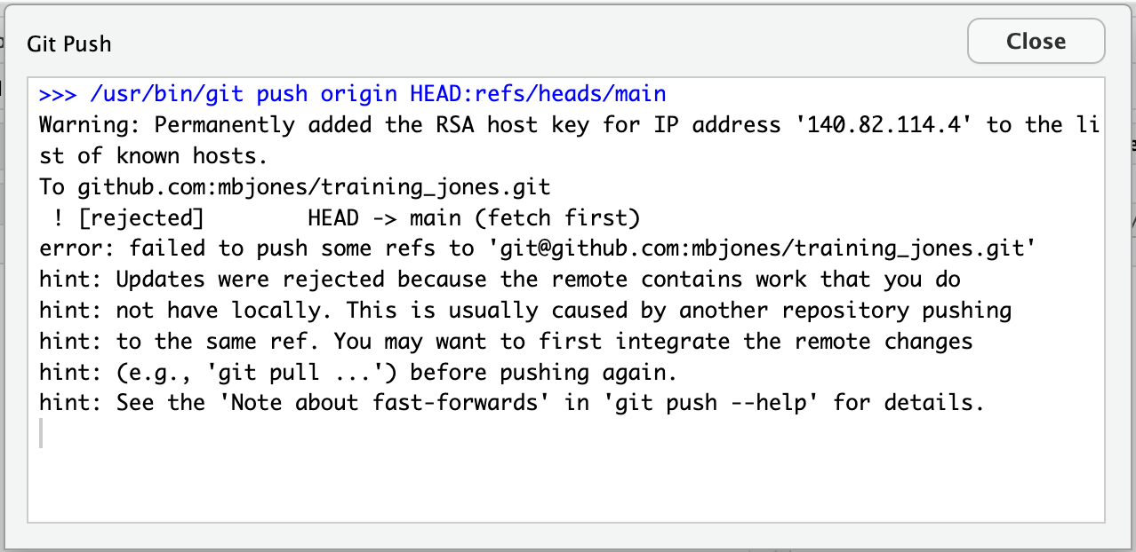
5.8.5.1.6 Owner pulls from GitHub to get Collaborator changes
Doing what the message says, the Owner pulls the changes from GitHub, and gets another, different error message. In this case, it indicates that there is a merge conflict because of the conflicting lines.
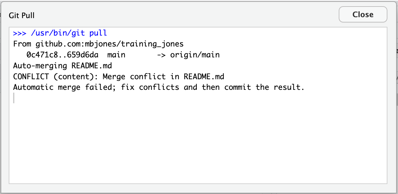
In the Git pane of RStudio, the file is also flagged with an orange ‘U’, which stands for an unresolved merge conflict.
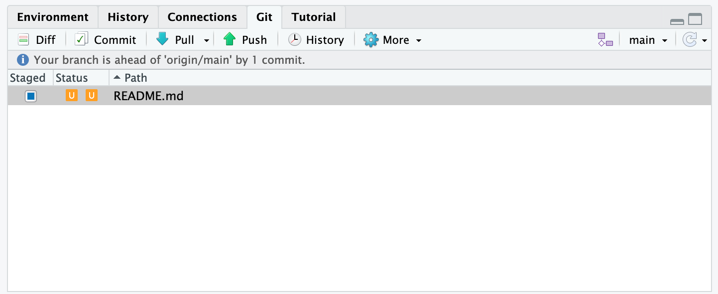
5.8.5.1.7 Owner edits the file to resolve the conflict
To resolve the conflict, the Owner now needs to edit the file. Again, as indicated above,
git has flagged the locations in the file where a conflict occcurred
with <<<<<<<, =======, and >>>>>>>. The Owner should edit the file, merging whatever
changes are appropriate until the conflicting lines read how they should, and eliminate
all of the marker lines with with <<<<<<<, =======, and >>>>>>>.
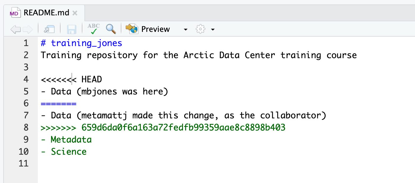
Of course, for scripts and programs, resolving the changes means more than just merging the text – whoever is doing the merging should make sure that the code runs properly and none of the logic of the program has been broken.
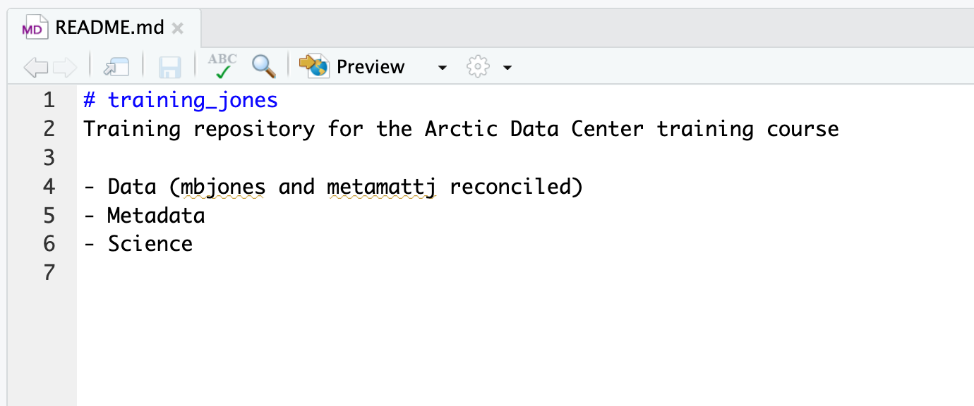
5.8.5.1.8 Owner commits the resolved changes
From this point forward, things proceed as normal. The owner first ‘Adds’ the file
changes to be made, which changes the orange U to a blue M for modified, and then
commits the changes locally. The owner now has a resolved version of the file on their
system.
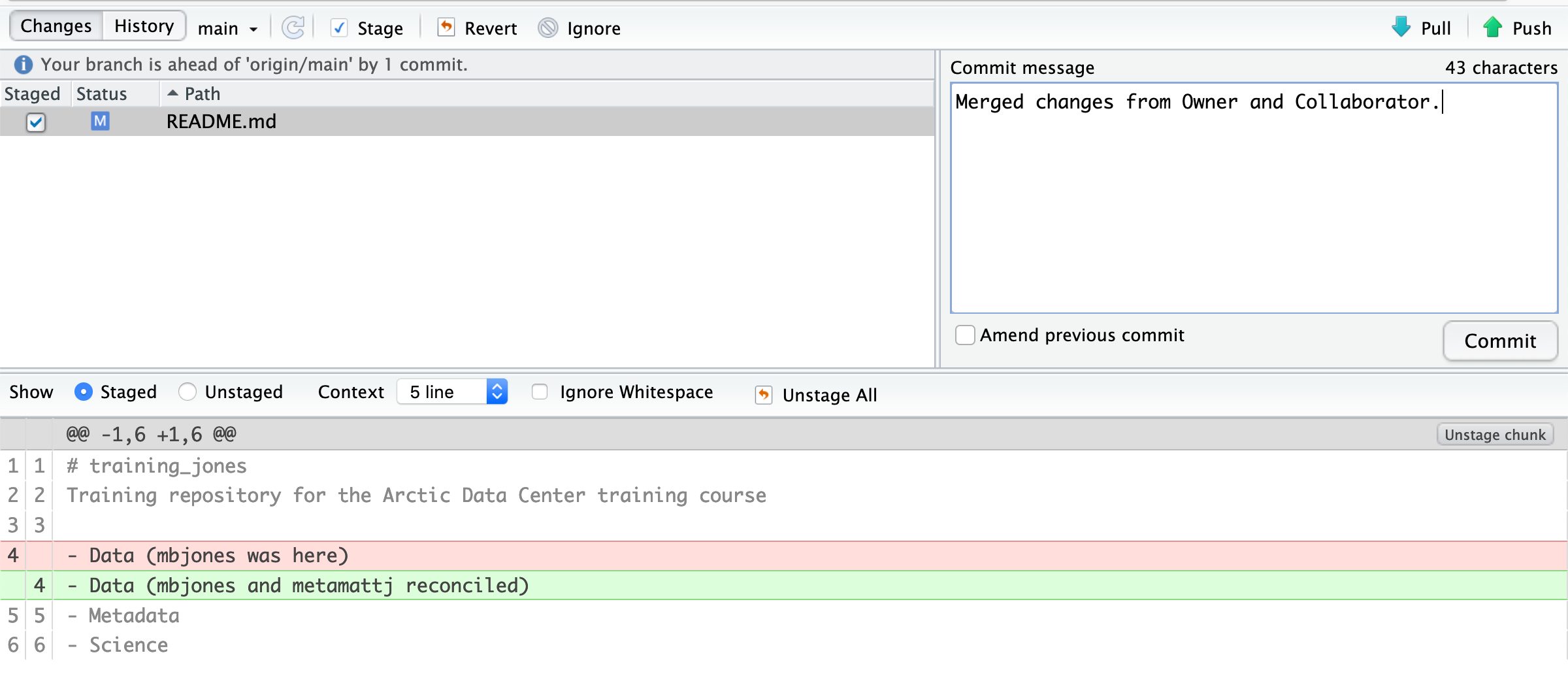
5.8.5.1.9 Owner pushes the resolved changes to GitHub
Have the Owner push the changes, and it should replicate the changes to GitHub without error.
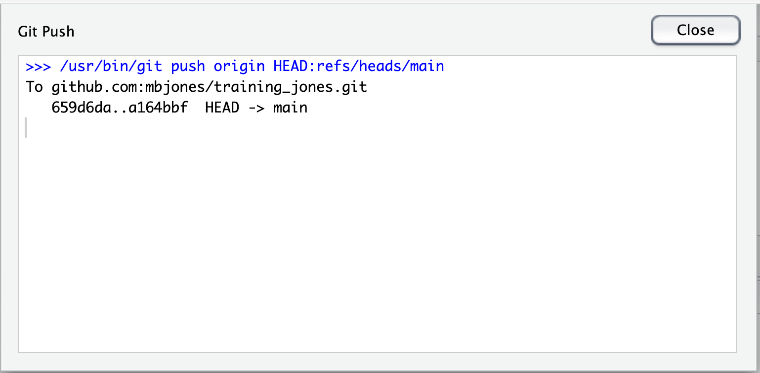
5.8.5.1.10 Collaborator pulls the resolved changes from GitHub
Finally, the Collaborator can pull from GitHub to get the changes the owner made.
5.8.5.1.11 Both can view commit history
When either the Collaborator or the Owner view the history, the conflict, associated branch, and the merged changes are clearly visible in the history.
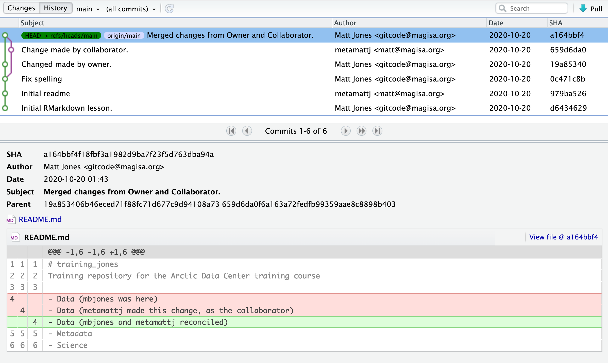
Merge Conflict Challenge
Now it’s your turn. With your partner, intentionally create a merge conflict, and then go through the steps needed to resolve the issues and continue developing with the merged files. See the sections above for help with each of these steps:
- Step 0: Owner and collaborator ensure all changes are updated
- Step 1: Owner makes a change and commits
- Step 2: Collaborator makes a change and commits on the same line
- Step 3: Collaborator pushes the file to GitHub
- Step 4: Owner pushes their changes and gets an error
- Step 5: Owner pulls from GitHub to get Collaborator changes
- Step 6: Owner edits the file to resolve the conflict
- Step 7: Owner commits the resolved changes
- Step 8: Owner pushes the resolved changes to GitHub
- Step 9: Collaborator pulls the resolved changes from GitHub
- Step 10: Both can view commit history
5.8.6 Workflows to avoid merge conflicts
Some basic rules of thumb can avoid the vast majority of merge conflicts, saving a lot of time and frustration. These are words our teams live by:
- Communicate often
- Tell each other what you are working on
- Pull immediately before you commit or push
- Commit often in small chunks.
A good workflow is encapsulated as follows:
Pull -> Edit -> Add -> Pull -> Commit -> Push
Always start your working sessions with a pull to get any outstanding changes, then start doing your editing and work. Stage your changes, but before you commit, Pull again to see if any new changes have arrived. If so, they should merge in easily if you are working in different parts of the program. You can then Commit and immediately Push your changes safely. Good luck, and try to not get frustrated. Once you figure out how to handle merge conflicts, they can be avoided or dispatched when they occur, but it does take a bit of practice.
5.9 Data Modeling & Tidy Data
5.9.1 Learning Objectives
- Understand basics of relational data models aka tidy data
- Learn how to design and create effective data tables
5.9.2 Introduction
In this lesson we are going to learn what relational data models are, and how they can be used to manage and analyze data efficiently. Relational data models are what relational databases use to organize tables. However, you don’t have to be using a relational database (like mySQL, MariaDB, Oracle, or Microsoft Access) to enjoy the benefits of using a relational data model. Additionally, your data don’t have to be large or complex for you to benefit. Here are a few of the benefits of using a relational data model:
- Powerful search and filtering
- Handle large, complex data sets
- Enforce data integrity
- Decrease errors from redundant updates
Simple guidelines for data management
A great paper called ‘Some Simple Guidelines for Effective Data Management’ (Borer et al. 2009) lays out exactly that - guidelines that make your data management, and your reproducible research, more effective. The first six guidelines are straightforward, but worth mentioning here:
- Use a scripted program (like R!)
- Non-proprietary file formats are preferred (eg: csv, txt)
- Keep a raw version of data
- Use descriptive file and variable names (without spaces!)
- Include a header line in your tabular data files
- Use plain ASCII text
The next three are a little more complex, but all are characteristics of the relational data model:
- Design tables to add rows, not columns
- Each column should contain only one type of information
- Record a single piece of data only once; separate information collected at different scales into different tables.
5.9.3 Recognizing untidy data
Before we learn how to create a relational data model, let’s look at how to recognize data that does not conform to the model.
Data Organization
This is a screenshot of an actual dataset that came across NCEAS. We have all seen spreadsheets that look like this - and it is fairly obvious that whatever this is, it isn’t very tidy. Let’s dive deeper in to exactly why we wouldn’t consider it tidy.
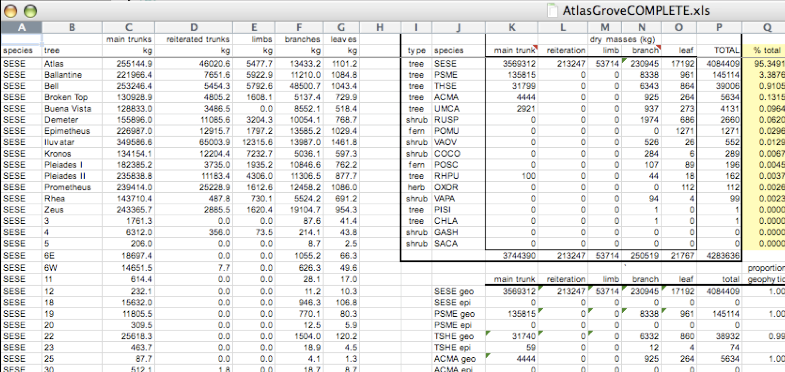
Multiple tables
Your human brain can see from the way this sheet is laid out that it has three tables within it. Although it is easy for us to see and interpret this, it is extremely difficult to get a computer to see it this way, which will create headaches down the road should you try to read in this information to R or another programming language.
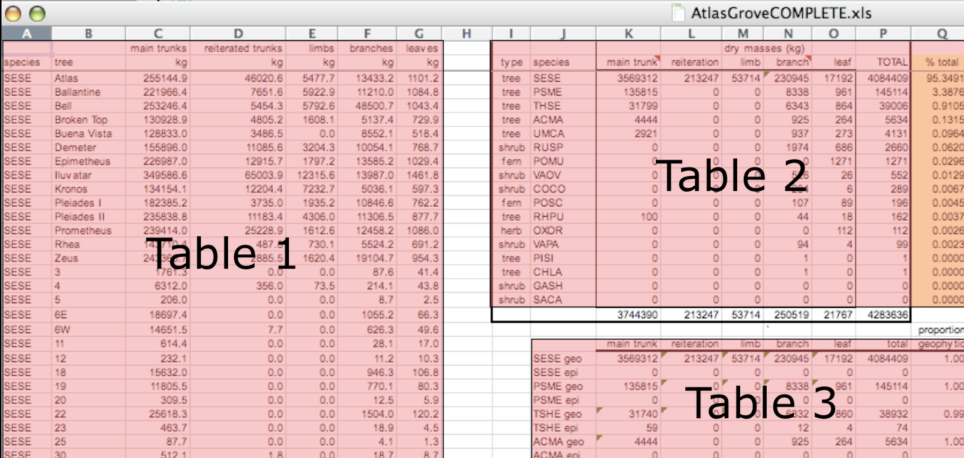
Inconsistent observations
Rows correspond to observations. If you look across a single row, and you notice that there are clearly multiple observations in one row, the data are likely not tidy.
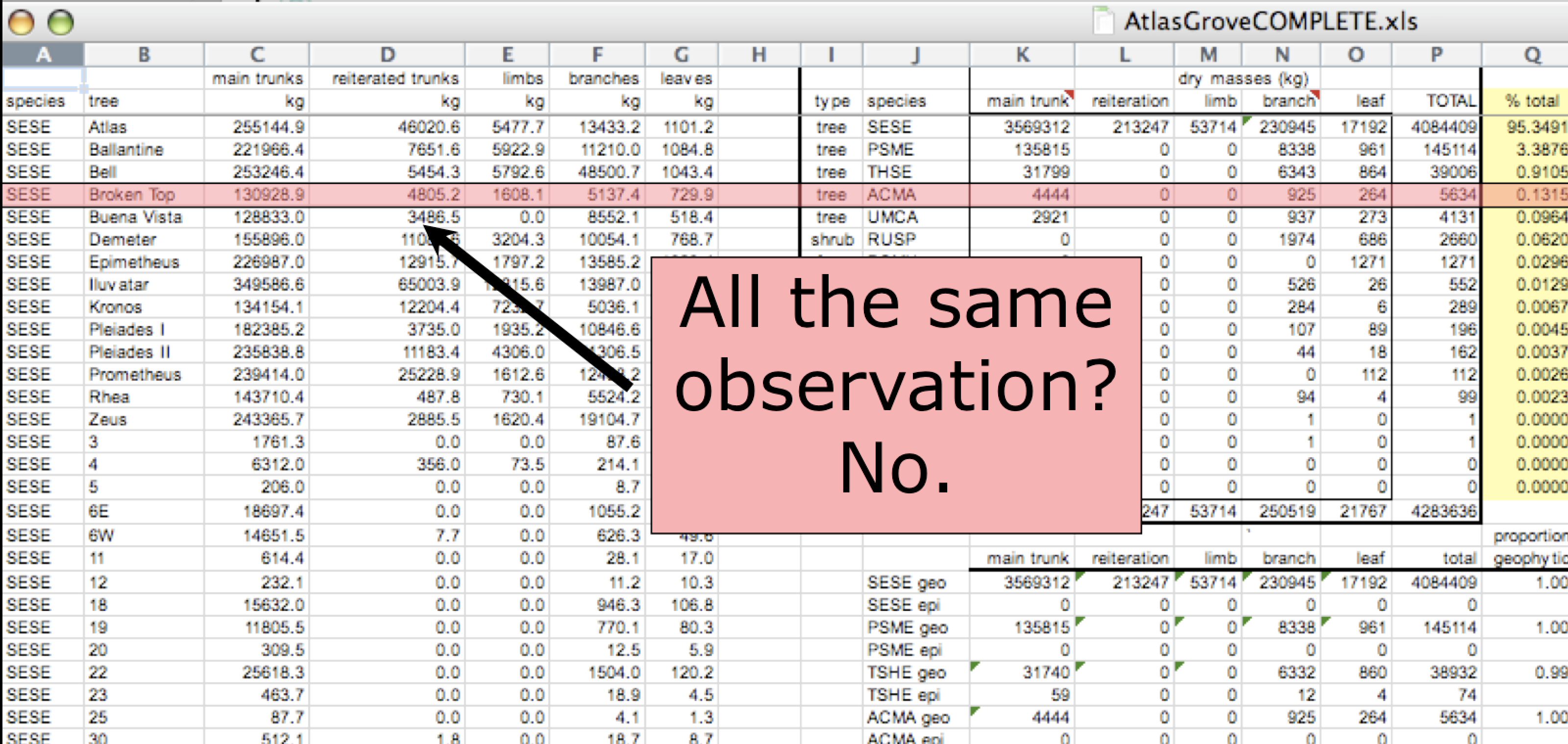
Inconsistent variables
Columns correspond to variables. If you look down a column, and see that multiple variables exist in the table, the data are not tidy. A good test for this can be to see if you think the column consists of only one unit type.
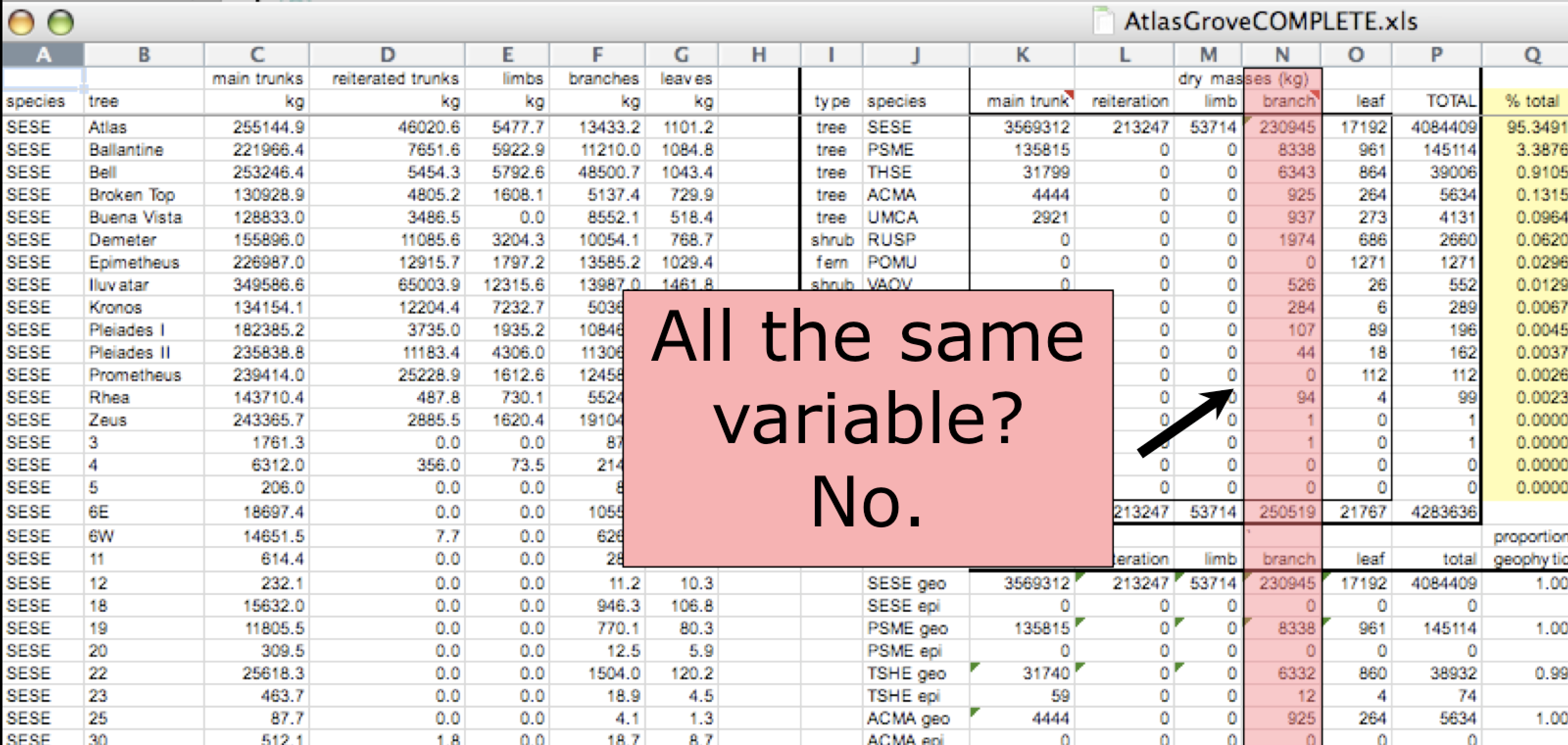
Marginal sums and statistics
Marginal sums and statistics also are not considered tidy, and they are not the same type of observation as the other rows. Instead, they are a combination of observations.
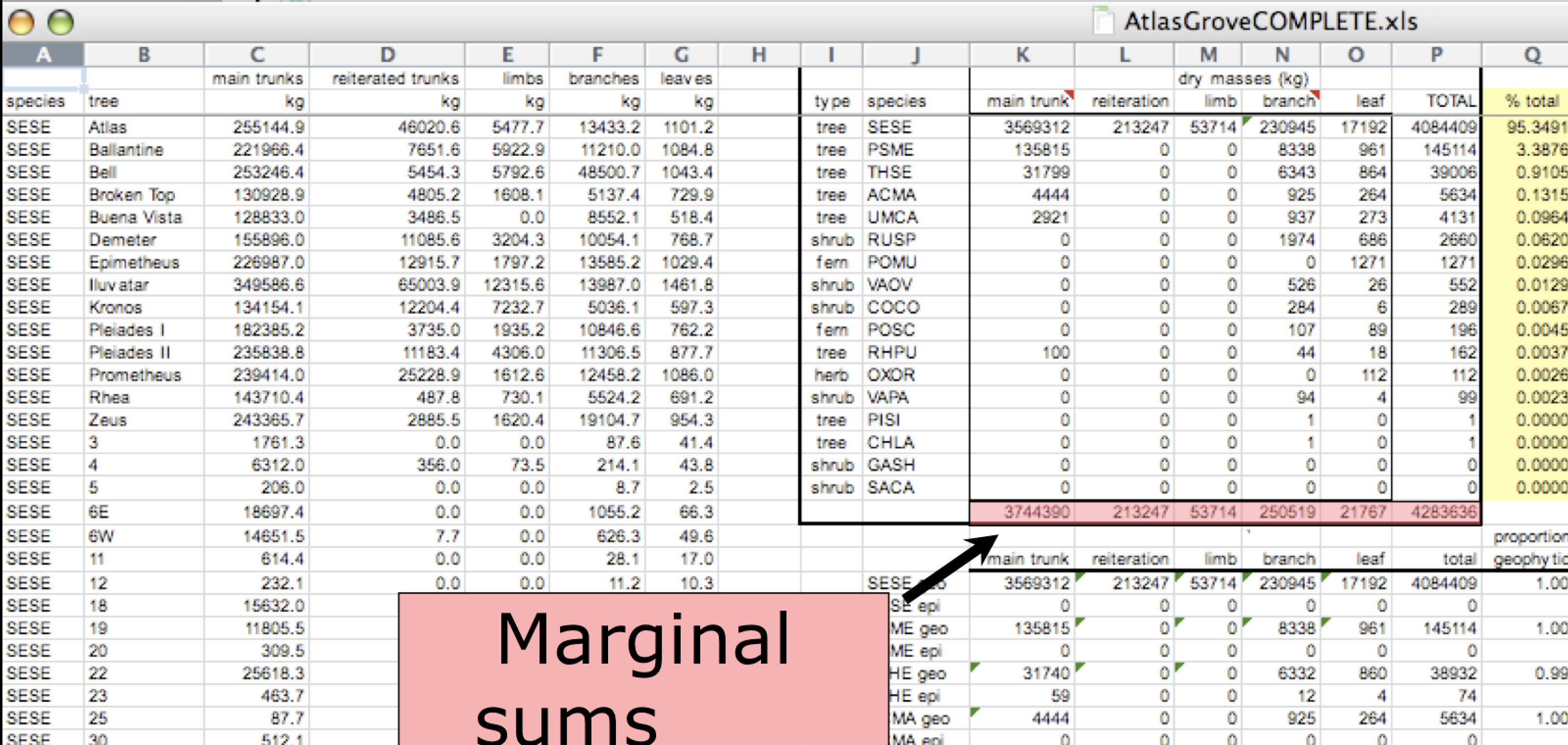
5.9.4 Good enough data modeling
Denormalized data
When data are “denormalized” it means that observations about different entities are combined.
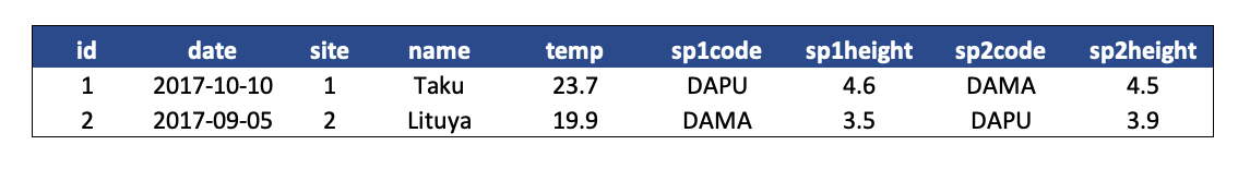
In the above example, each row has measurements about both the site at which observations occurred, as well as observations of two individuals of possibly different species found at that site. This is not normalized data.
People often refer to this as wide format, because the observations are spread across a wide number of columns. Note that, should one encounter a new species in the survey, we wold have to add new columns to the table. This is difficult to analyze, understand, and maintain.
Tabular data
Observations. A better way to model data is to organize the observations about each type of entity in its own table. This results in:
Separate tables for each type of entity measured
Each row represents a single observed entity
Observations (rows) are all unique
This is normalized data (aka tidy data)
Variables. In addition, for normalized data, we expect the variables to be organized such that:
- All values in a column are of the same type
- All columns pertain to the same observed entity (e.g., row)
- Each column represents either an identifying variable or a measured variable
Challenge
Try to answer the following questions:
What are the observed entities in the example above?
What are the measured variables associated with those observations?
Answer:
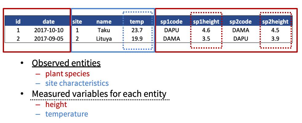
If we use these questions to tidy our data, we should end up with:
- one table for each entity observed
- one column for each measured variable
- additional columns for identifying variables (such as site ID)
Here is what our tidy data look like:
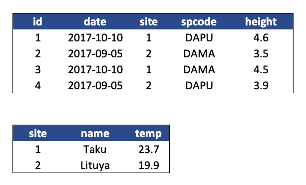
Note that this normalized version of the data meets the three guidelines set by (Borer et al. 2009):
- Design tables to add rows, not columns
- Each column should contain only one type of information
- Record a single piece of data only once; separate information collected at different scales into different tables.
5.9.5 Using normalized data
Normalizing data by separating it into multiple tables often makes researchers really uncomfortable. This is understandable! The person who designed this study collected all of these measurements for a reason - so that they could analyze the measurements together. Now that our site and species information are in separate tables, how would we use site elevation as a predictor variable for species composition, for example? The answer is keys - and they are the cornerstone of relational data models.
When one has normalized data, we often use unique identifiers to reference particular observations, which allows us to link across tables. Two types of identifiers are common within relational data:
- Primary Key: unique identifier for each observed entity, one per row
- Foreign Key: reference to a primary key in another table (linkage)
Challenge
In our normalized tables above, identify the following:
- the primary key for each table
- any foreign keys that exist
Answer
The primary key of the top table is id. The primary key of the bottom table is site.
The site column is the primary key of that table because it uniquely identifies each row of the table as a unique observation of a site. In the first table, however, the site column is a foreign key that references the primary key from the second table. This linkage tells us that the first height measurement for the DAPU observation occurred at the site with the name Taku.
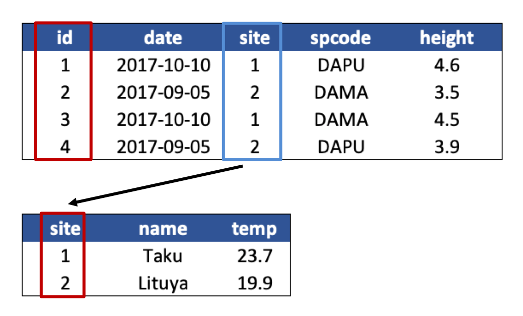
Entity-Relationship Model (ER)
An Entity-Relationship model allows us to compactly draw the structure of the tables in a relational database, including the primary and foreign keys in the tables.
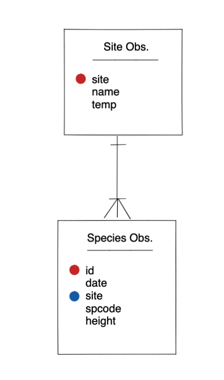
In the above model, one can see that each site in the sites observations table must have one or more observations in the species observations table, whereas each species opservation has one and only one site.
Merging data
Frequently, analysis of data will require merging these separately managed tables back together. There are multiple ways to join the observations in two tables, based on how the rows of one table are merged with the rows of the other.
When conceptualizing merges, one can think of two tables, one on the left and one on the right. The most common (and often useful) join is when you merge the subset of rows that have matches in both the left table and the right table: this is called an INNER JOIN. Other types of join are possible as well. A LEFT JOIN takes all of the rows from the left table, and merges on the data from matching rows in the right table. Keys that don’t match from the left table are still provided with a missing value (na) from the right table. A RIGHT JOIN is the same, except that all of the rows from the right table are included with matching data from the left, or a missing value. Finally, a FULL OUTER JOIN includes all data from all rows in both tables, and includes missing values wherever necessary.
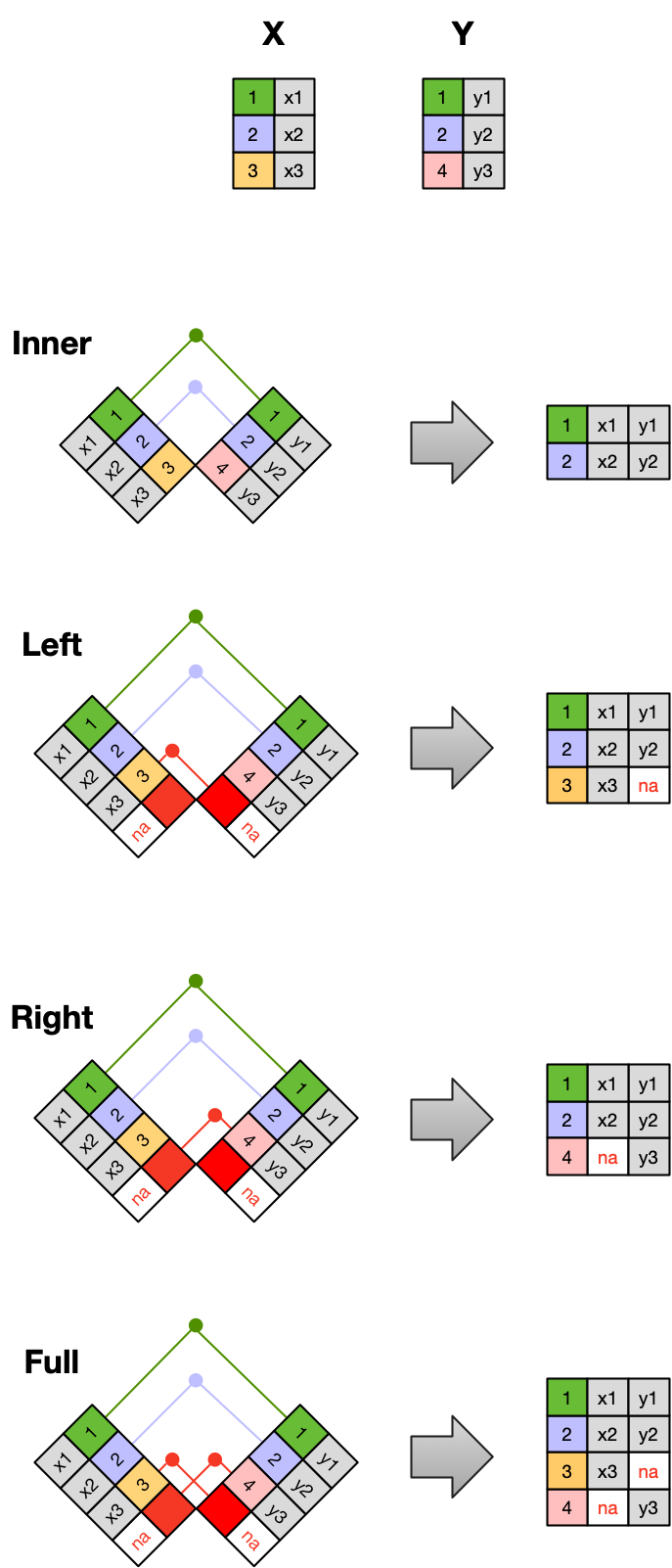
Sometimes people represent these as Venn diagrams showing which parts of the left and right tables are included in the results for each join. These however, miss part of the story related to where the missing value come from in each result.
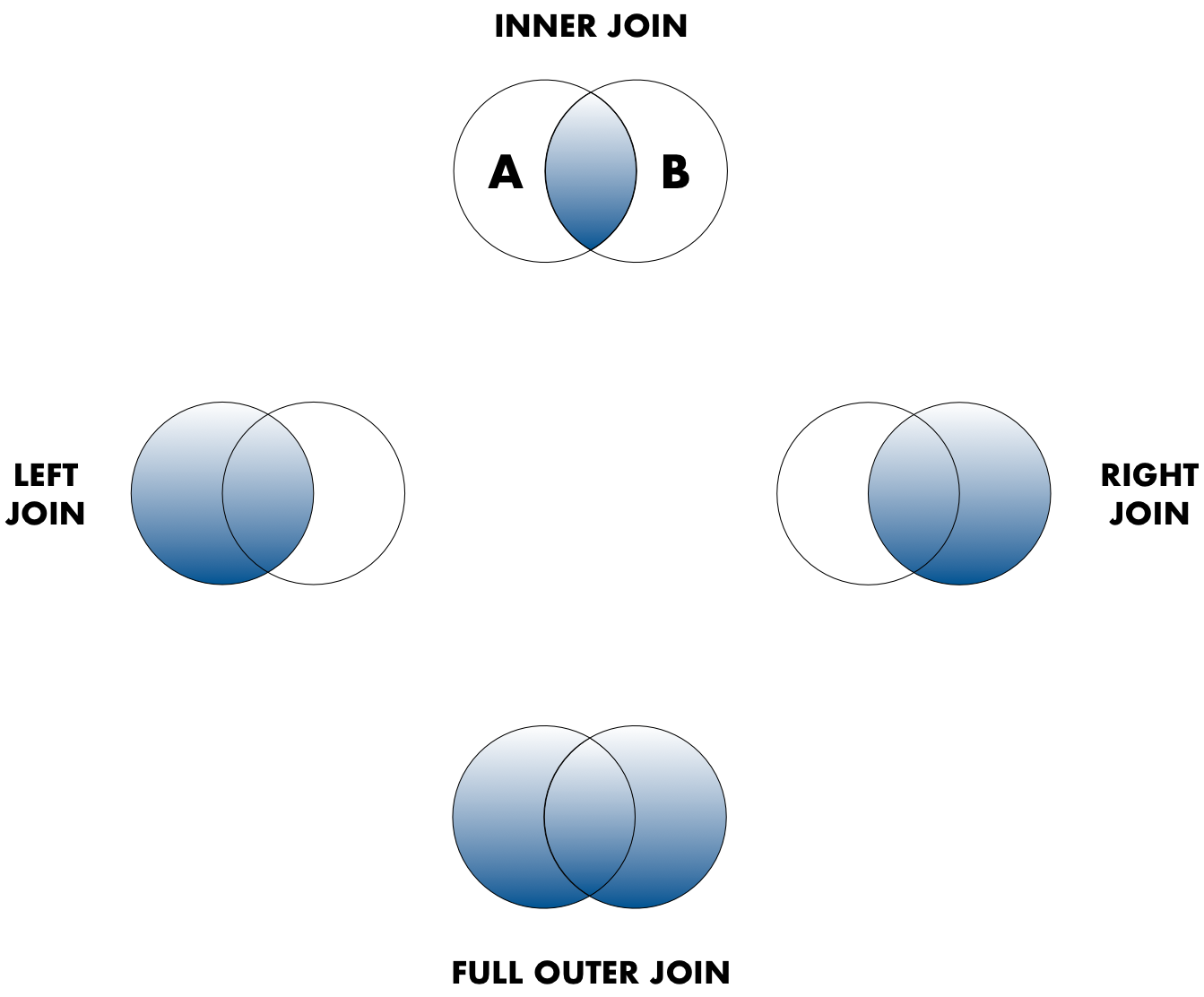
In the figure above, the blue regions show the set of rows that are included in the result. For the INNER join, the rows returned are all rows in A that have a matching row in B.
5.9.6 Data modeling exercise
You may choose to do this exercise in a group with your lab, or individually.
To demonstrate, we’ll be working with a tidied up version of a dataset from ADF&G containing commercial catch data from 1878-1997. The dataset and reference to the original source can be viewed at its public archive: https://knb.ecoinformatics.org/#view/df35b.304.2. That site includes metadata describing the full data set, including column definitions. Here’s the first catch table:
And here’s the region_defs table:
Challenge
Work through the following tasks:
Draw an ER model for the tables
- Indicate the primary and foreign keys
Is the
catchtable in normal (aka tidy) form?If so, what single type of entity was observed?
If not, how might you restructure the data table to make it tidy?
- Draw a new ER diatram showing this re-designed data structure
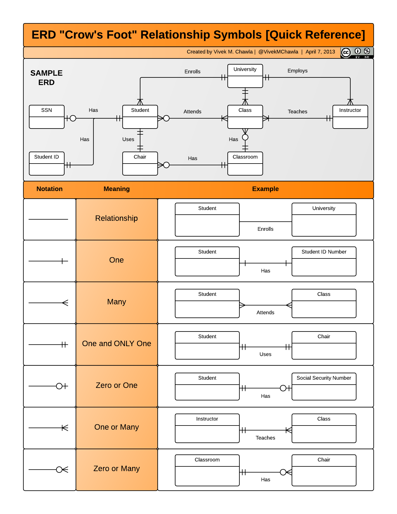
Optional Extra Challenge
If you have time, take on this extra challenge.
Navigate to this dataset: Richard Lanctot and Sarah Saalfeld. 2019. Utqiaġvik shorebird breeding ecology study, Utqiaġvik, Alaska, 2003-2018. Arctic Data Center. doi:10.18739/A23R0PT35
Try to determine the primary and foreign keys for the following tables:
- Utqiagvik_adult_shorebird_banding.csv
- Utqiagvik_egg_measurements.csv
- Utqiagvik_nest_data.csv
- Utqiagvik_shorebird_resightings.csv
5.10 Data Cleaning and Manipulation
5.10.1 Learning Objectives
In this lesson, you will learn:
- What the Split-Apply-Combine strategy is and how it applies to data
- The difference between wide vs. tall table formats and how to convert between them
- How to use
dplyrandtidyrto clean and manipulate data for analysis - How to join multiple
data.frames together usingdplyr
5.10.2 Introduction
The data we get to work with are rarely, if ever, in the format we need to do our analyses. It’s often the case that one package requires data in one format, while another package requires the data to be in another format. To be efficient analysts, we should have good tools for reformatting data for our needs so we can do our actual work like making plots and fitting models. The dplyr and tidyr R packages provide a fairly complete and extremely powerful set of functions for us to do this reformatting quickly and learning these tools well will greatly increase your efficiency as an analyst.
Analyses take many shapes, but they often conform to what is known as the Split-Apply-Combine strategy. This strategy follows a usual set of steps:
- Split: Split the data into logical groups (e.g., area, stock, year)
- Apply: Calculate some summary statistic on each group (e.g. mean total length by year)
- Combine: Combine the groups back together into a single table
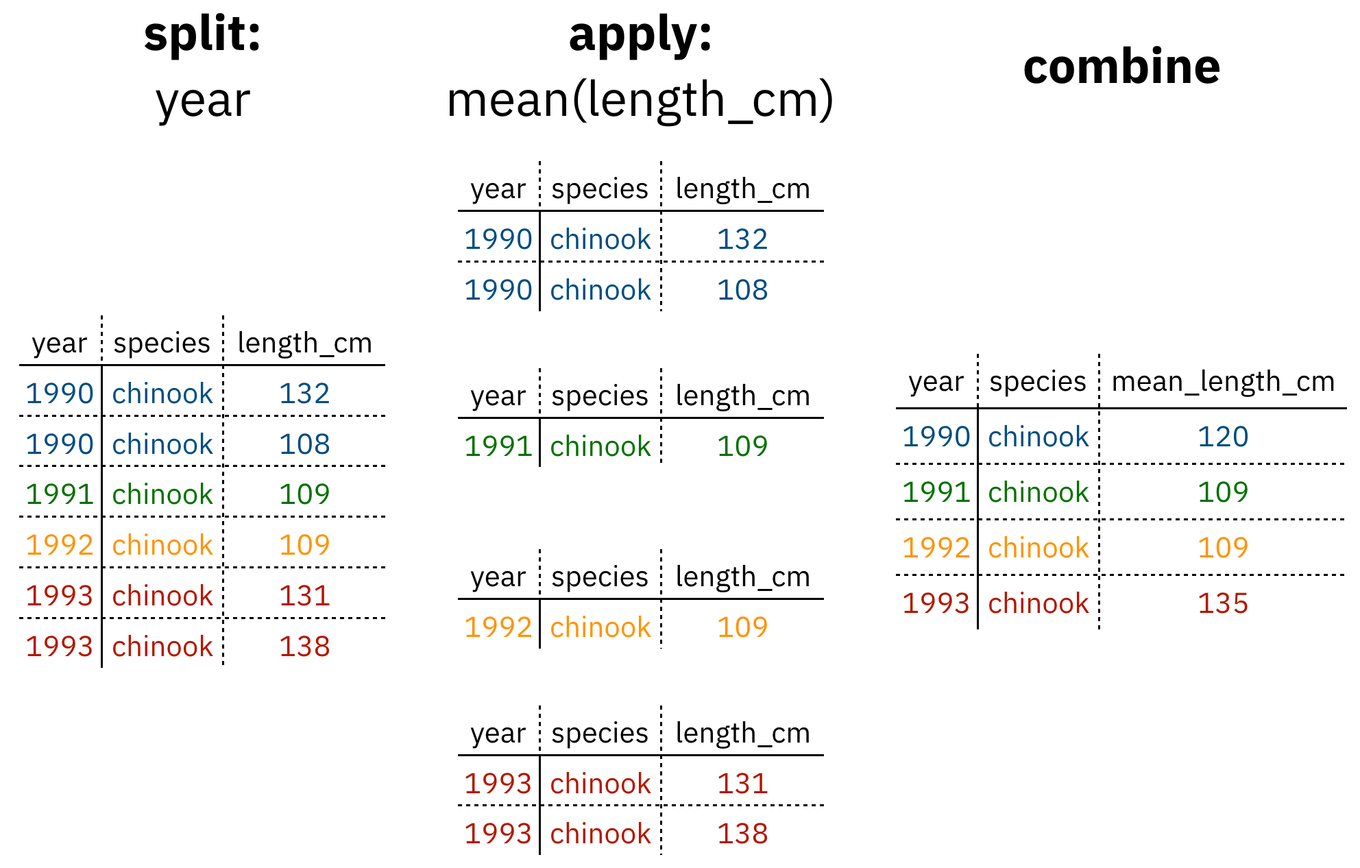
Figure 1: diagram of the split apply combine strategy
As shown above (Figure 1), our original table is split into groups by year, we calculate the mean length for each group, and finally combine the per-year means into a single table.
dplyr provides a fast and powerful way to express this. Let’s look at a simple example of how this is done:
Assuming our length data is already loaded in a data.frame called length_data:
| year | length_cm |
|---|---|
| 1991 | 5.673318 |
| 1991 | 3.081224 |
| 1991 | 4.592696 |
| 1992 | 4.381523 |
| 1992 | 5.597777 |
| 1992 | 4.900052 |
| 1992 | 4.139282 |
| 1992 | 5.422823 |
| 1992 | 5.905247 |
| 1992 | 5.098922 |
We can do this calculation using dplyr like this:
Another exceedingly common thing we need to do is “reshape” our data. Let’s look at an example table that is in what we will call “wide” format:
| site | 1990 | 1991 | … | 1993 |
|---|---|---|---|---|
| gold | 100 | 118 | … | 112 |
| lake | 100 | 118 | … | 112 |
| … | … | … | … | … |
| dredge | 100 | 118 | … | 112 |
You are probably quite familiar with data in the above format, where values of the variable being observed are spread out across columns (Here: columns for each year). Another way of describing this is that there is more than one measurement per row. This wide format works well for data entry and sometimes works well for analysis but we quickly outgrow it when using R. For example, how would you fit a model with year as a predictor variable? In an ideal world, we’d be able to just run:
But this won’t work on our wide data because lm needs length and year to be columns in our table.
Or how would we make a separate plot for each year? We could call plot one time for each year but this is tedious if we have many years of data and hard to maintain as we add more years of data to our dataset.
The tidyr package allows us to quickly switch between wide format and what is called tall format using the pivot_longer function:
| site | year | length |
|---|---|---|
| gold | 1990 | 101 |
| lake | 1990 | 104 |
| dredge | 1990 | 144 |
| … | … | … |
| dredge | 1993 | 145 |
In this lesson we’re going to walk through the functions you’ll most commonly use from the dplyr and tidyr packages:
dplyrmutate()group_by()summarise()select()filter()arrange()left_join()rename()
tidyrpivot_longer()pivot_wider()extract()separate()
5.10.3 Data Cleaning Basics
To demonstrate, we’ll be working with a tidied up version of a dataset from ADF&G containing commercial catch data from 1878-1997. The dataset and reference to the original source can be found at its public archive: https://knb.ecoinformatics.org/#view/df35b.304.2.
First, open a new RMarkdown document. Delete everything below the setup chunk, and add a library chunk that calls dplyr, tidyr, and readr:
Aside
A note on loading packages.
You may have noticed the following warning messages pop up when you ran your library chunk.
Attaching package: ‘dplyr’

The following objects are masked from ‘package:stats’:

    filter, lag

The following objects are masked from ‘package:base’:

    intersect, setdiff, setequal, union
These are important warnings. They are letting you know that certain functions from the stats and base packages (which are loaded by default when you start R) are masked by different functions with the same name in the dplyr package. It turns out, the order that you load the packages in matters. Since we loaded dplyr after stats, R will assume that if you call filter, you mean the dplyr version unless you specify otherwise.
Being specific about which version of filter, for example, you call is easy. To explicitly call a function by its unambiguous name, you use the syntax package_name::function_name(...). So, if I wanted to call the stats version of filter in this Rmarkdown document, I would use the syntax stats::filter(...).
Challenge
The warnings above are important, but we might not want them in our final document. After you have read them, adjust the chunk settings on your library chunk to suppress warnings and messages.
Now that we have learned a little mini-lesson on functions, let’s get the data that we are going to use for this lesson.
Setup
Navigate to the salmon catch dataset: https://knb.ecoinformatics.org/#view/df35b.304.2
Right click the “download” button for the file “byerlySalmonByRegion.csv”
Select “copy link address” from the dropdown menu
Paste the URL into a
read_csvcall like below
The code chunk you use to read in the data should look something like this:
Aside
Note that windows users who want to use this method locally also need to use the url function here with the argument method = "libcurl" as below:
This dataset is relatively clean and easy to interpret as-is. But while it may be clean, it’s in a shape that makes it hard to use for some types of analyses so we’ll want to fix that first.
Challenge
Before we get too much further, spend a minute or two outlining your RMarkdown document so that it includes the following sections and steps:
- Data Sources
- read in the data
- Clean and Reshape data
- remove unnecessary columns
- check column typing
- reshape data
- Join to Regions dataset
About the pipe (%>%) operator
Before we jump into learning tidyr and dplyr, we first need to explain the %>%.
Both the tidyr and the dplyr packages use the pipe operator - %>%, which may look unfamiliar. The pipe is a powerful way to efficiently chain together operations. The pipe will take the output of a previous statement, and use it as the input to the next statement.
Say you want to both filter out rows of a dataset, and select certain columns. Instead of writing
df_filtered <- filter(df, ...)
df_selected <- select(df_filtered, ...)
You can write
df_cleaned <- df %>%
              filter(...) %>%
              select(...)
If you think of the assignment operator (<-) as reading like “gets”, then the pipe operator would read like “then.”
So you might think of the above chunk being translated as:
The cleaned dataframe gets the original data, and then a filter (of the original data), and then a select (of the filtered data).
The benefits to using pipes are that you don’t have to keep track of (or overwrite) intermediate data frames. The drawbacks are that it can be more difficult to explain the reasoning behind each step, especially when many operations are chained together. It is good to strike a balance between writing efficient code (chaining operations), while ensuring that you are still clearly explaining, both to your future self and others, what you are doing and why you are doing it.
RStudio has a keyboard shortcut for %>% : Ctrl + Shift + M (Windows), Cmd + Shift + M (Mac).
Selecting/removing columns: select()
The first issue is the extra columns All and notesRegCode. Let’s select only the columns we want, and assign this to a variable called catch_data.
catch_data <- catch_original %>%
  select(Region, Year, Chinook, Sockeye, Coho, Pink, Chum)

head(catch_data)
## # A tibble: 6 x 7
## Region Year Chinook Sockeye Coho Pink Chum
## <chr> <dbl> <chr> <dbl> <dbl> <dbl> <dbl>
## 1 SSE 1886 0 5 0 0 0
## 2 SSE 1887 0 155 0 0 0
## 3 SSE 1888 0 224 16 0 0
## 4 SSE 1889 0 182 11 92 0
## 5 SSE 1890 0 251 42 0 0
## 6 SSE 1891 0 274 24 0 0Much better!
select also allows you to say which columns you don’t want, by passing unquoted column names preceded by minus (-) signs:
## # A tibble: 6 x 7
##   Region  Year Chinook Sockeye  Coho  Pink  Chum
##   <chr>  <dbl> <chr>     <dbl> <dbl> <dbl> <dbl>
## 1 SSE     1886 0             5     0     0     0
## 2 SSE     1887 0           155     0     0     0
## 3 SSE     1888 0           224    16     0     0
## 4 SSE     1889 0           182    11    92     0
## 5 SSE     1890 0           251    42     0     0
## 6 SSE 1891 0 274 24 0 0Quality Check
Now that we have the data we are interested in using, we should do a little quality check to see that it seems as expected. One nice way of doing this is the summary function.
##     Region               Year        Chinook
##  Length:1708        Min.   :1878   Length:1708
##  Class :character   1st Qu.:1922   Class :character
##  Mode  :character   Median :1947   Mode  :character
##                     Mean   :1946
##                     3rd Qu.:1972
##                     Max.   :1997
##     Sockeye              Coho             Pink
##  Min.   :    0.00   Min.   :   0.0   Min.   :    0.0
##  1st Qu.:    6.75   1st Qu.:   0.0   1st Qu.:    0.0
##  Median :  330.50   Median :  41.5   Median :   34.5
##  Mean   : 1401.09   Mean   : 150.4   Mean   : 2357.8
##  3rd Qu.:  995.50   3rd Qu.: 175.0   3rd Qu.: 1622.5
##  Max.   :44269.00   Max.   :3220.0   Max.   :53676.0
##       Chum
##  Min.   :    0.0
##  1st Qu.:    0.0
##  Median :   63.0
##  Mean   :  422.0
##  3rd Qu.:  507.5
##  Max.   :10459.0
Challenge
Notice the output of the summary function call. Does anything seem amiss with this dataset that might warrant fixing?
Answer: The Chinook catch data are character class. Let’s fix it using the function mutate before moving on.
Changing column content: mutate()
We can use the mutate function to change a column, or to create a new column. First Let’s try to just convert the Chinook catch values to numeric type using the as.numeric() function, and overwrite the old Chinook column.
## Warning: Problem with `mutate()` input `Chinook`.
## ℹ NAs introduced by coercion
## ℹ Input `Chinook` is `as.numeric(Chinook)`.
## Warning in mask$eval_all_mutate(dots[[i]]): NAs
## introduced by coercion## # A tibble: 6 x 7
## Region Year Chinook Sockeye Coho Pink Chum
## <chr> <dbl> <dbl> <dbl> <dbl> <dbl> <dbl>
## 1 SSE 1886 0 5 0 0 0
## 2 SSE 1887 0 155 0 0 0
## 3 SSE 1888 0 224 16 0 0
## 4 SSE 1889 0 182 11 92 0
## 5 SSE 1890 0 251 42 0 0
## 6 SSE 1891 0 274 24 0 0We get a warning “NAs introduced by coercion” which is R telling us that it couldn’t convert every value to an integer and, for those values it couldn’t convert, it put an NA in its place. This is behavior we commonly experience when cleaning datasets and it’s important to have the skills to deal with it when it crops up.
To investigate, let’s isolate the issue. We can find out which values are NAs with a combination of is.na() and which(), and save that to a variable called i.
## [1] 401It looks like there is only one problem row, lets have a look at it in the original data.
## # A tibble: 1 x 7
##   Region  Year Chinook Sockeye  Coho  Pink  Chum
##   <chr>  <dbl> <chr>     <dbl> <dbl> <dbl> <dbl>
## 1 GSE     1955 I            66     0     0     1
Well that’s odd: The value in catch_thousands is I. It turns out that this dataset is from a PDF which was automatically converted into a CSV and this value of I is actually a 1.
Let’s fix it by incorporating the ifelse function to our mutate call, which will change the value of the Chinook column to 1 if the value is equal to I, otherwise it will leave the column as the same value.
catch_clean <- catch_data %>%
  mutate(Chinook = ifelse(Chinook == "I", 1, Chinook)) %>%
  mutate(Chinook = as.integer(Chinook))

head(catch_clean)
## # A tibble: 6 x 7
## Region Year Chinook Sockeye Coho Pink Chum
## <chr> <dbl> <int> <dbl> <dbl> <dbl> <dbl>
## 1 SSE 1886 0 5 0 0 0
## 2 SSE 1887 0 155 0 0 0
## 3 SSE 1888 0 224 16 0 0
## 4 SSE 1889 0 182 11 92 0
## 5 SSE 1890 0 251 42 0 0
## 6 SSE 1891 0 274 24 0 0Changing shape: pivot_longer() and pivot_wider()
The next issue is that the data are in a wide format and, we want the data in a tall format instead. pivot_longer() from the tidyr package helps us do just this conversion:
catch_long <- catch_clean %>%
  pivot_longer(cols = -c(Region, Year), names_to = "species", values_to = "catch")

head(catch_long)
## # A tibble: 6 x 4
## Region Year species catch
## <chr> <dbl> <chr> <dbl>
## 1 SSE 1886 Chinook 0
## 2 SSE 1886 Sockeye 5
## 3 SSE 1886 Coho 0
## 4 SSE 1886 Pink 0
## 5 SSE 1886 Chum 0
## 6 SSE 1887 Chinook 0The syntax we used above for pivot_longer() might be a bit confusing so let’s walk though it.
The first argument to pivot_longer is the columns over which we are pivoting. You can select these by listing either the names of the columns you do want to pivot, or the names of the columns you are not pivoting over. The names_to argument takes the name of the column that you are creating from the column names you are pivoting over. The values_to argument takes the name of the column that you are creating from the values in the columns you are pivoting over.
The opposite of pivot_longer(), pivot_wider(), works in a similar declarative fashion:
catch_wide <- catch_long %>%
  pivot_wider(names_from = species, values_from = catch)

head(catch_wide)
## # A tibble: 6 x 7
## Region Year Chinook Sockeye Coho Pink Chum
## <chr> <dbl> <dbl> <dbl> <dbl> <dbl> <dbl>
## 1 SSE 1886 0 5 0 0 0
## 2 SSE 1887 0 155 0 0 0
## 3 SSE 1888 0 224 16 0 0
## 4 SSE 1889 0 182 11 92 0
## 5 SSE 1890 0 251 42 0 0
## 6 SSE 1891 0 274 24 0 0Renaming columns with rename()
If you scan through the data, you may notice the values in the catch column are very small (these are supposed to be annual catches). If we look at the metadata we can see that the catch column is in thousands of fish so let’s convert it before moving on.
Let’s first rename the catch column to be called catch_thousands:
## # A tibble: 6 x 4
##   Region  Year species catch_thousands
##   <chr>  <dbl> <chr>             <dbl>
## 1 SSE     1886 Chinook               0
## 2 SSE     1886 Sockeye               5
## 3 SSE     1886 Coho                  0
## 4 SSE     1886 Pink                  0
## 5 SSE     1886 Chum                  0
## 6 SSE     1887 Chinook               0
Aside
Many people use the base R function names to rename columns, often in combination with column indexing that relies on columns being in a particular order. Column indexing is often also used to select columns instead of the select function from dplyr. Although these methods both work just fine, they do have one major drawback: in most implementations they rely on you knowing exactly the column order your data is in.
To illustrate why your knowledge of column order isn’t reliable enough for these operations, considering the following scenario:
Your colleague emails you letting you know that she has an updated version of the conductivity-temperature-depth data from this year’s research cruise, and sends it along. Excited, you re-run your scripts that use this data for your phytoplankton research. You run the script and suddenly all of your numbers seem off. You spend hours trying to figure out what is going on.
Unbeknownst to you, your colleagues bought a new sensor this year that measures dissolved oxygen. Because of the new variables in the dataset, the column order is different. Your script which previously renamed the 4th column, SAL_PSU to salinity now renames the 4th column, O2_MGpL to salinity. No wonder your results looked so weird, good thing you caught it!
If you had written your code so that it doesn’t rely on column order, but instead renames columns using the rename function, the code would have run just fine (assuming the name of the original salinity column didn’t change, in which case the code would have errored in an obvious way). This is an example of a defensive coding strategy, where you try to anticipate issues before they arise, and write your code in such a way as to keep the issues from happening.
Adding columns: mutate()
Now let’s use mutate again to create a new column called catch with units of fish (instead of thousands of fish).
Now let’s remove the catch_thousands column for now since we don’t need it. Note that here we have added to the expression we wrote above by adding another function call (mutate) to our expression. This takes advantage of the pipe operator by grouping together a similar set of statements, which all aim to clean up the catch_long data.frame.
catch_long <- catch_long %>%
  mutate(catch = catch_thousands * 1000) %>%
  select(-catch_thousands)

head(catch_long)
## # A tibble: 6 x 4
## Region Year species catch
## <chr> <dbl> <chr> <dbl>
## 1 SSE 1886 Chinook 0
## 2 SSE 1886 Sockeye 5000
## 3 SSE 1886 Coho 0
## 4 SSE 1886 Pink 0
## 5 SSE 1886 Chum 0
## 6 SSE 1887 Chinook 0We’re now ready to start analyzing the data.
group_by and summarise
As I outlined in the Introduction, dplyr lets us employ the Split-Apply-Combine strategy and this is exemplified through the use of the group_by() and summarise() functions:
## `summarise()` ungrouping output (override with `.groups` argument)## # A tibble: 6 x 2
## Region catch_mean
## <chr> <dbl>
## 1 ALU 40384.
## 2 BER 16373.
## 3 BRB 2709796.
## 4 CHG 315487.
## 5 CKI 683571.
## 6 COP 179223.Another common use of group_by() followed by summarize() is to count the number of rows in each group. We have to use a special function from dplyr, n().
## `summarise()` ungrouping output (override with `.groups` argument)## # A tibble: 6 x 2
## Region n
## <chr> <int>
## 1 ALU 435
## 2 BER 510
## 3 BRB 570
## 4 CHG 550
## 5 CKI 525
## 6 COP 470Challenge
- Find another grouping and statistic to calculate for each group.
- Find out if you can group by multiple variables.
Filtering rows: filter()
filter() is the verb we use to filter our data.frame to rows matching some condition. It’s similar to subset() from base R.
Let’s go back to our original data.frame and do some filter()ing:
## # A tibble: 6 x 4
##   Region  Year species catch
##   <chr>  <dbl> <chr>   <dbl>
## 1 SSE     1886 Chinook     0
## 2 SSE     1886 Sockeye  5000
## 3 SSE     1886 Coho        0
## 4 SSE     1886 Pink        0
## 5 SSE     1886 Chum        0
## 6 SSE 1887 Chinook 0Challenge
- Filter to just catches of over one million fish.
- Filter to just Chinook from the SSE region
Sorting your data: arrange()
arrange() is how we sort the rows of a data.frame. In my experience, I use arrange() in two common cases:
- When I want to calculate a cumulative sum (with
cumsum()) so row order matters - When I want to display a table (like in an
.Rmddocument) in sorted order
Let’s re-calculate mean catch by region, and then arrange() the output by mean catch:
mean_region <- catch_long %>%
  group_by(Region) %>%
  summarise(mean_catch = mean(catch)) %>%
  arrange(mean_catch)
## `summarise()` ungrouping output (override with `.groups` argument)## # A tibble: 6 x 2
## Region mean_catch
## <chr> <dbl>
## 1 BER 16373.
## 2 KTZ 18836.
## 3 ALU 40384.
## 4 NRS 51503.
## 5 KSK 67642.
## 6 YUK 68646.The default sorting order of arrange() is to sort in ascending order. To reverse the sort order, wrap the column name inside the desc() function:
mean_region <- catch_long %>%
  group_by(Region) %>%
  summarise(mean_catch = mean(catch)) %>%
  arrange(desc(mean_catch))
## `summarise()` ungrouping output (override with `.groups` argument)## # A tibble: 6 x 2
## Region mean_catch
## <chr> <dbl>
## 1 SSE 3184661.
## 2 BRB 2709796.
## 3 NSE 1825021.
## 4 KOD 1528350
## 5 PWS 1419237.
## 6 SOP 1110942.5.10.4 Joins in dplyr
So now that we’re awesome at manipulating a single data.frame, where do we go from here? Manipulating more than one data.frame.
If you’ve ever used a database, you may have heard of or used what’s called a “join”, which allows us to to intelligently merge two tables together into a single table based upon a shared column between the two. We’ve already covered joins in Data Modeling & Tidy Data so let’s see how it’s done with dplyr.
The dataset we’re working with, https://knb.ecoinformatics.org/#view/df35b.304.2, contains a second CSV which has the definition of each Region code. This is a really common way of storing auxiliary information about our dataset of interest (catch) but, for analylitcal purposes, we often want them in the same data.frame. Joins let us do that easily.
Let’s look at a preview of what our join will do by looking at a simplified version of our data:
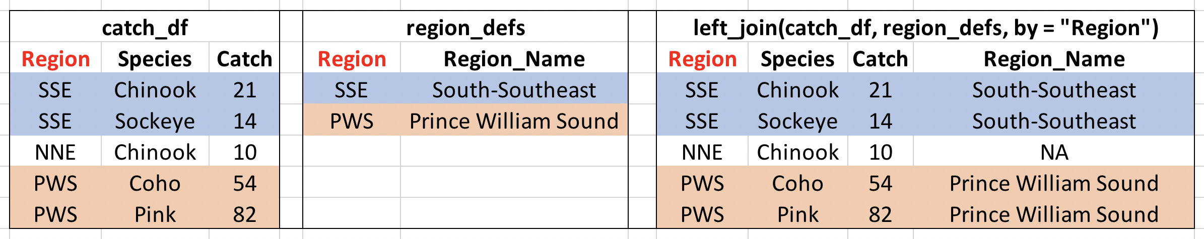
Visualisation of our left_join
First, let’s read in the region definitions data table and select only the columns we want. Note that I have piped my read.csv result into a select call, creating a tidy chunk that reads and selects the data that we need.
region_defs <- read_csv("https://knb.ecoinformatics.org/knb/d1/mn/v2/object/df35b.303.1") %>%
    select(code, mgmtArea)
## Parsed with column specification:
## cols(
## code = col_character(),
## mgmtArea = col_character(),
## areaClass = col_character(),
## regionCode = col_double(),
## notes = col_character()
## )## # A tibble: 6 x 2
## code mgmtArea
## <chr> <chr>
## 1 GSE Unallocated Southeast Alaska
## 2 NSE Northern Southeast Alaska
## 3 SSE Southern Southeast Alaska
## 4 YAK Yakutat
## 5 PWSmgmt Prince William Sound Management Area
## 6 BER Bering River Subarea Copper River SubareaIf you examine the region_defs data.frame, you’ll see that the column names don’t exactly match the image above. If the names of the key columns are not the same, you can explicitly specify which are the key columns in the left and right side as shown below:
## # A tibble: 6 x 5
##   Region  Year species catch mgmtArea
##   <chr>  <dbl> <chr>   <dbl> <chr>
## 1 SSE     1886 Chinook     0 Southern Southeast Alaska
## 2 SSE     1886 Sockeye  5000 Southern Southeast Alaska
## 3 SSE     1886 Coho        0 Southern Southeast Alaska
## 4 SSE     1886 Pink        0 Southern Southeast Alaska
## 5 SSE     1886 Chum        0 Southern Southeast Alaska
## 6 SSE     1887 Chinook     0 Southern Southeast Alaska
Notice that I have deviated from our usual pipe syntax (although it does work here!) because I prefer to see the data.frames that I am joining side by side in the syntax.
Another way you can do this join is to use rename to change the column name code to Region in the region_defs data.frame, and run the left_join this way:
region_defs <- region_defs %>%
  rename(Region = code, Region_Name = mgmtArea)

catch_joined <- left_join(catch_long, region_defs, by = c("Region"))

head(catch_joined)
Now our catches have the auxiliary information from the region definitions file alongside them. Note: dplyr provides a complete set of joins: inner, left, right, full, semi, anti, not just left_join.
separate() and unite()
separate() and its complement, unite() allow us to easily split a single column into numerous (or numerous into a single).
This can come in really handle when we need to split a column into two pieces by a consistent separator (like a dash).
Let’s make a new data.frame with fake data to illustrate this. Here we have a set of site identification codes. with information about the island where the site is (the first 3 letters) and a site number (the 3 numbers). If we want to group and summarize by island, we need a column with just the island information.
sites_df <- data.frame(site = c("HAW-101",
                                "HAW-103",
                                "OAH-320",
                                "OAH-219",
                                "MAI-039"),
                       stringsAsFactors = FALSE)

sites_df %>%
  separate(site, c("island", "site_number"), "-")
## island site_number
## 1 HAW 101
## 2 HAW 103
## 3 OAH 320
## 4 OAH 219
## 5 MAI 039- Exercise: Split the
citycolumn in the followingdata.frameintocityandstate_codecolumns:
cities_df <- data.frame(city = c("Juneau AK",
                                 "Sitka AK",
                                 "Anchorage AK"),
                        stringsAsFactors = FALSE)

# Write your solution here
unite() does just the reverse of separate(). If we have a data.frame that contains columns for year, month, and day, we might want to unite these into a single date column.
dates_df <- data.frame(year = c("1930",
                                "1930",
                                "1930"),
                       month = c("12",
                                "12",
                                "12"),
                       day = c("14",
                               "15",
                               "16"),
                       stringsAsFactors = FALSE)

dates_df %>%
  unite(date, year, month, day, sep = "-")
## date
## 1 1930-12-14
## 2 1930-12-15
## 3 1930-12-16- Exercise: Use
unite()on your solution above to combine thecities_dfback to its original form with just one column,city:
Summary
We just ran through the various things we can do with dplyr and tidyr but if you’re wondering how this might look in a real analysis. Let’s look at that now:
catch_original <- read.csv(url("https://knb.ecoinformatics.org/knb/d1/mn/v2/object/df35b.302.1", method = "libcurl"),
                  stringsAsFactors = FALSE)
region_defs <- read.csv(url("https://knb.ecoinformatics.org/knb/d1/mn/v2/object/df35b.303.1", method = "libcurl"),
                        stringsAsFactors = FALSE) %>%
    select(code, mgmtArea)

mean_region <- catch_original %>%
  select(-All, -notesRegCode) %>%
  mutate(Chinook = ifelse(Chinook == "I", 1, Chinook)) %>%
  mutate(Chinook = as.numeric(Chinook)) %>%
  pivot_longer(-c(Region, Year), names_to = "species", values_to = "catch") %>%
  mutate(catch = catch*1000) %>%
  group_by(Region) %>%
  summarize(mean_catch = mean(catch)) %>%
  left_join(region_defs, by = c("Region" = "code"))
## `summarise()` ungrouping output (override with `.groups` argument)## # A tibble: 6 x 3
## Region mean_catch mgmtArea
## <chr> <dbl> <chr>
## 1 ALU 40384. Aleutian Islands Subarea
## 2 BER 16373. Bering River Subarea Copper River …
## 3 BRB 2709796. Bristol Bay Management Area
## 4 CHG 315487. Chignik Management Area
## 5 CKI 683571. Cook Inlet Management Area
## 6 COP 179223. Copper River Subarea5.11 Publishing Analyses to the Web
5.11.1 Learning Objectives
In this lesson, you will learn:
- How to use git, GitHub (+Pages), and (R)Markdown to publish an analysis to the web
5.11.2 Introduction
Sharing your work with others in engaging ways is an important part of the scientific process. So far in this course, we’ve introduced a small set of powerful tools for doing open science:
- R and its many packages
- RStudio
- git
- GiHub
- RMarkdown
RMarkdown, in particular, is amazingly powerful for creating scientific reports but, so far, we haven’t tapped its full potential for sharing our work with others.
In this lesson, we’re going to take an existing GitHub repository and turn it into a beautiful and easy to read web page using the tools listed above.
5.11.3 A Minimal Example
- Use your existing
training_usernamerepository - Add a new file at the top level called
index.Rmd. The easiest way to do this is through the RStudio menu. Choose File -> New File -> RMarkdown… This will bring up a dialog box. You should create a “Document” in “HTML” format. These are the default options. Be sure to use the exact capitalization (lower case ‘index’) as different operating systems handle capitalization differently and it can interfere with loading your web page later. - Open
index.Rmd(if it isn’t already open) - Press Knit
- Observe the rendered output
- Notice the new file in the same directory
index.html. - This is our RMarkdown file rendered as HTML (a web page)
- Commit your changes (to both index.Rmd and index.html) and push to GitHub
- Open your web browser to the GitHub.com page for your repository
- Go to Settings > GitHub Pages and turn on GitHub Pages for the
masterbranch
Now, the rendered website version of your repo will show up at a special URL.
GitHub Pages follows a convention like this:
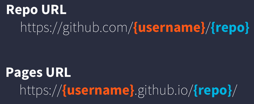
github pages url pattern
Note that it will no longer be at github.com but github.io
- Go to https://{username}.github.io/{repo_name}/ (Note the trailing
/) Observe the awesome rendered output
Now that we’ve successfully published a web page from an RMarkdown document, let’s make a change to our RMarkdown document and follow the steps to actually publish the change on the web:
- Go back to our
index.Rmd - Delete all the content, except the YAML frontmatter
- Type “Hello world”
- Commit, push
- Go back to https://{username}.github.io/{repo_name}/
5.11.4 Exercise: Sharing your work
RMarkdown web pages are a great way to share work in progress with your colleagues. To do so simply requires thinking through your presentation so that it highlights the workflow to be reviewed. You can also include multiple pages and build a simple web site for walking through your work that is accessible to people who aren’t all set up to open your content in R. In this exercise, we’ll publish another RMarkdown page, and create a table of contents on the main page to guide people to the main page.
First, in your trainnig repository, create a new RMarkdown file that describes some piece of your work and note the name. I’ll use an RMarkdown named data-cleaning.Rmd.
Once you have an RMarkdown created, Knit the document which will create the HTML version of the file, which in this case will be named data-cleaning.html.
Now, return to editing your index.Rmd file from the beginning of this lesson. The index file represents the ‘default’ file for a web site, and is returned whenever you visit the web site but don’t specify an explicit file to be returned. Let’s modify the index page, adding a bulleted list, and in that list, include a link to the new markdown page that we created:
## Analysis plan

- [Data Cleaning](data-cleaning.html)
- Data Interpolation and Gap filling
- Linear models
- Animal movement models based on telemetry
- Data visualization
Commit and push the web page to GitHub. Now when you visit your web site, you’ll see the table of contents, and can navigate to the new data cleaning page.
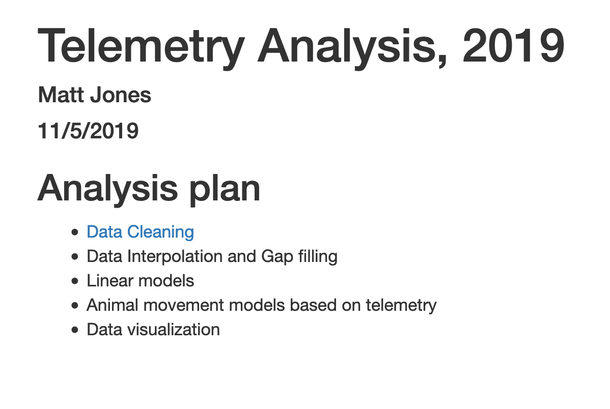
5.12 Creating R Functions
Many people write R code as a single, continuous stream of commands, often drawn
from the R Console itself and simply pasted into a script. While any script
brings benefits over non-scripted solutions, there are advantages to breaking
code into small, reusable modules. This is the role of a function in R. In
this lesson, we will review the advantages of coding with functions, practice
by creating some functions and show how to call them, and then do some exercises
to build other simple functions.
5.12.0.1 Learning outcomes
- Learn why we should write code in small functions
- Write code for one or more functions
- Document functions to improve understanding and code communication
5.12.1 Why functions?
In a word:
- DRY: Don’t Repeat Yourself
By creating small functions that only one logical task and do it well, we quickly gain:
- Improved understanding
- Reuse via decomposing tasks into bite-sized chunks
- Improved error testing
Temperature conversion
Imagine you have a bunch of data measured in Fahrenheit and you want to convert that for analytical purposes to Celsius. You might have an R script that does this for you.
airtemps <- c(212, 30.3, 78, 32)
celsius1 <- (airtemps[1]-32)*5/9
celsius2 <- (airtemps[2]-32)*5/9
celsius3 <- (airtemps[3]-32)*5/9
Note the duplicated code, where the same formula is repeated three times. This code would be both more compact and more reliable if we didn’t repeat ourselves.
Creating a function
Functions in R are a mechanism to process some input and return a value. Similarly
to other variables, functions can be assigned to a variable so that they can be used
throughout code by reference. To create a function in R, you use the function function (so meta!) and assign its result to a variable. Let’s create a function that calculates
celsius temperature outputs from fahrenheit temperature inputs.
By running this code, we have created a function and stored it in R’s global environment. The fahr argument to the function function indicates that the function we are creating takes a single parameter (the temperature in fahrenheit), and the return statement indicates that the function should return the value in the celsius variable that was calculated inside the function. Let’s use it, and check if we got the same value as before:
## [1] 100## [1] TRUEExcellent. So now we have a conversion function we can use. Note that, because
most operations in R can take multiple types as inputs, we can also pass the original vector of airtemps, and calculate all of the results at once:
## [1] 100.0000000 -0.9444444 25.5555556 0.0000000This takes a vector of temperatures in fahrenheit, and returns a vector of temperatures in celsius.
Challenge
Now, create a function named celsius_to_fahr that does the reverse, it takes temperature data in celsius as input, and returns the data converted to fahrenheit. Then use that formula to convert the celsius vector back into a vector of fahrenheit values, and compare it to the original airtemps vector to ensure that your answers are correct. Hint: the formula for C to F conversions is celsius*9/5 + 32.
Did you encounter any issues with rounding or precision?
5.12.2 Documenting R functions
Functions need documentation so that we can communicate what they do, and why. The roxygen2 package provides a simple means to document your functions so that you can explain what the function does, the assumptions about the input values, a description of the value that is returned, and the rationale for decisions made about implementation.
Documentation in ROxygen is placed immediately before the function definition, and is indicated by a special comment line that always starts with the characters #'. Here’s a documented version of a function:
#' Convert temperature data from Fahrenheit to Celsius
#'
#' @param fahr Temperature data in degrees Fahrenheit to be converted
#' @return temperature value in degrees Celsius
#' @keywords conversion
#' @export
#' @examples
#' fahr_to_celsius(32)
#' fahr_to_celsius(c(32, 212, 72))
fahr_to_celsius <- function(fahr) {
  celsius <- (fahr-32)*5/9
  return(celsius)
}Note the use of the @param keyword to define the expectations of input data, and the @return keyword for defining the value that is returned from the function. The @examples function is useful as a reminder as to how to use the function. Finally, the @export keyword indicates that, if this function were added to a package, then the function should be available to other code and packages to utilize.
5.12.3 Summary
- Functions are useful to reduce redundancy, reuse code, and reduce errors
- Build functions with the
functionfunction - Document functions with
roxygen2comments
5.12.4 Examples: Minimizing work with functions
Functions can of course be as simple or complex as needed. They can be be very effective in repeatedly performing calculations, or for bundling a group of commands that are used on many different input data sources. For example, we might create a simple function that takes fahrenheit temperatures as input, and calculates both celsius and Kelvin temperatures. All three values are then returned in a list, making it very easy to create a comparison table among the three scales.
convert_temps <- function(fahr) {
  celsius <- (fahr-32)*5/9
  kelvin <- celsius + 273.15
  return(list(fahr=fahr, celsius=celsius, kelvin=kelvin))
}

temps_df <- data.frame(convert_temps(seq(-100,100,10)))
Once we have a dataset like that, we might want to plot it. One thing that we do
repeatedly is set a consistent set of display elements for creating graphs and plots.
By using a function to create a custom ggplot theme, we can enable to keep key
parts of the formatting flexible. FOr example, in the custom_theme function,
we provide a base_size argument that defaults to using a font size of 9 points.
Because it has a default set, it can safely be omitted. But if it is provided,
then that value is used to set the base font size for the plot.
custom_theme <- function(base_size = 9) {
    ggplot2::theme(
      axis.ticks       = ggplot2::element_blank(),
      text             = ggplot2::element_text(family = 'Helvetica', color = 'gray30', size = base_size),
      plot.title       = ggplot2::element_text(size = ggplot2::rel(1.25), hjust = 0.5, face = 'bold'),
      panel.background = ggplot2::element_blank(),
      legend.position  = 'right',
      panel.border     = ggplot2::element_blank(),
      panel.grid.minor = ggplot2::element_blank(),
      panel.grid.major = ggplot2::element_line(colour = 'grey90', size = .25),
      legend.key       = ggplot2::element_rect(colour = NA, fill = NA),
      axis.line        = ggplot2::element_blank()
      )
}

ggplot(temps_df, mapping=aes(x=fahr, y=celsius, color=kelvin)) +
    geom_point() +
    custom_theme(10)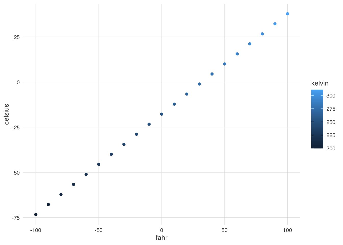
In this case, we set the font size to 10, and plotted the air temperatures. The custom_theme
function can be used anywhere that one needs to consistently format a plot.
But we can go further. One can wrap the entire call to ggplot in a function,
enabling one to create many plots of the same type with a consistent structure. For
example, we can create a scatterplot function that takes a data frame as input,
along with a point_size for the points on the plot, and a font_size for the text.
scatterplot <- function(df, point_size = 2, font_size=9) {
  ggplot(df, mapping=aes(x=fahr, y=celsius, color=kelvin)) +
    geom_point(size=point_size) +
    custom_theme(font_size)
}
Calling that let’s us, in a single line of code, create a highly customized plot but maintain flexibiity via the arguments passed in to the function. Let’s set the point size to 3 and font to 16 to make the plot more legible.
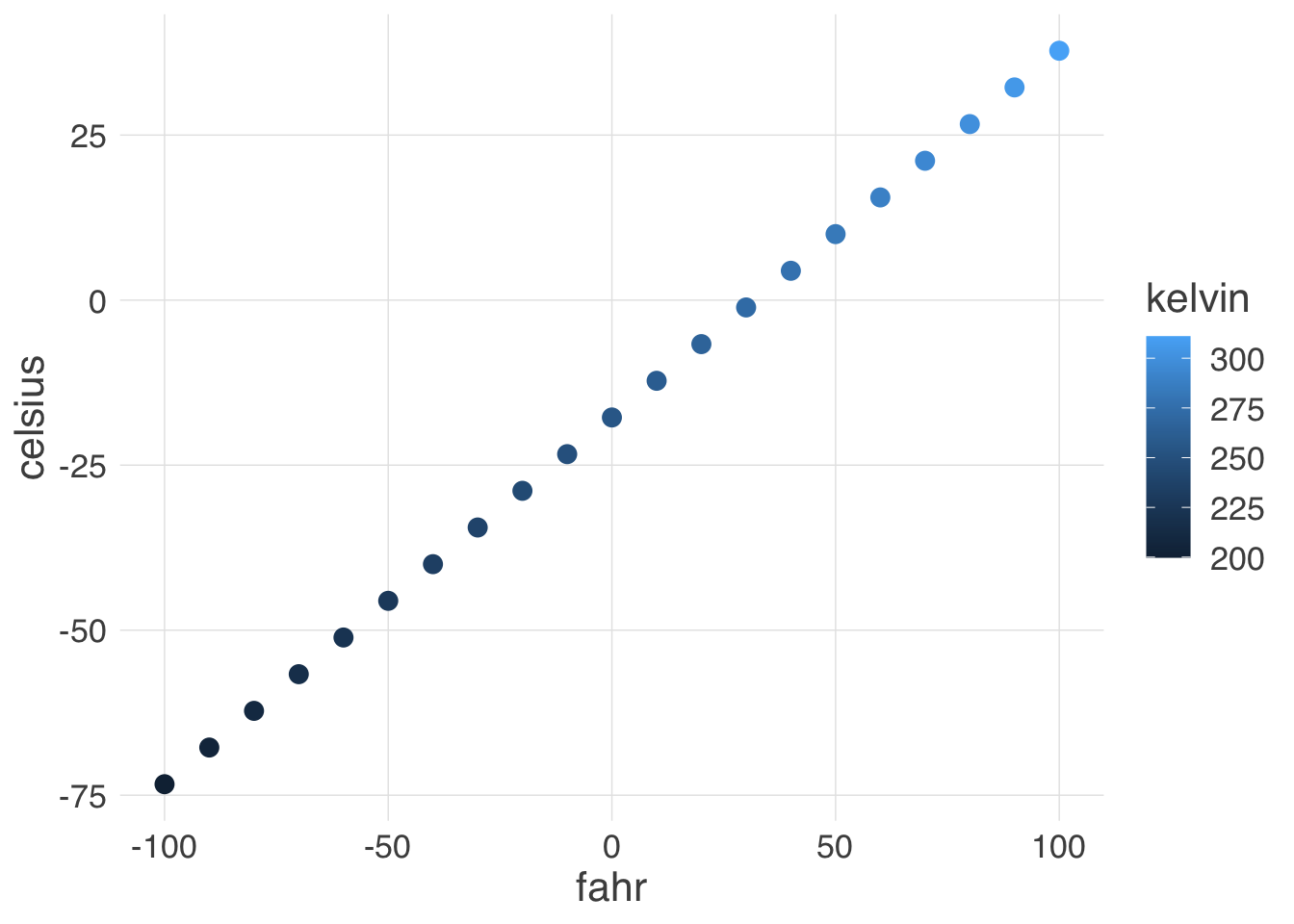
Once these functions are set up, all of the plots built with them can be reformatted by changing the settings in just the functions, whether they were used to create 1, 10, or 100 plots.
5.13 Creating R Packages
5.13.1 Learning Objectives
In this lesson, you will learn:
- The advantages of using R packages for organizing code
- Simple techniques for creating R packages
- Approaches to documenting code in packages
5.13.2 Why packages?
Most R users are familiar with loading and utilizing packages in their work. And they know how rich CRAN is in providing for many conceivable needs. Most people have never created a package for their own work, and most think the process is too complicated. Really it’s pretty straighforward and super useful in your personal work. Creating packages serves two main use cases:
- Mechanism to redistribute reusable code (even if just for yourself)
- Mechanism to reproducibly document analysis and models and their results
At a minimum, you can easily produce a package for just your own useful code functions, which makes it easy to maintain and use utilities that span your own projects.
The usethis, devtools and roxygen2 packages make creating and maintining a package to be a straightforward experience.
5.13.4 Create a basic package
Thanks to the great usethis package, it only takes one function call to create the skeleton of an R package using create_package(). Which eliminates pretty much all reasons for procrastination. To create a package called
mytools, all you do is:
✔ Setting active project to '/Users/jones/development/mytools'
✔ Creating 'R/'
✔ Creating 'man/'
✔ Writing 'DESCRIPTION'
✔ Writing 'NAMESPACE'
✔ Writing 'mytools.Rproj'
✔ Adding '.Rproj.user' to '.gitignore'
✔ Adding '^mytools\\.Rproj$', '^\\.Rproj\\.user$' to '.Rbuildignore'
✔ Opening new project 'mytools' in RStudio
Note that this will open a new project (mytools) and a new session in RStudio server.
The create_package function created a top-level directory structure, including a number of critical files under the standard R package structure. The most important of which is the DESCRIPTION file, which provides metadata about your package. Edit the DESCRIPTION file to provide reasonable values for each of the fields,
including your own contact information.
Information about choosing a LICENSE is provided in the Extending R documentation.
The DESCRIPTION file expects the license to be chose from a predefined list, but
you can use it’s various utility methods for setting a specific license file, such
as the Apacxhe 2 license:
✔ Setting License field in DESCRIPTION to 'Apache License (>= 2.0)'
✔ Writing 'LICENSE.md'
✔ Adding '^LICENSE\\.md$' to '.Rbuildignore'
Once your license has been chosen, and you’ve edited your DESCRIPTION file with your contact information, a title, and a description, it will look like this:
Package: mytools
Title: Utility Functions Created by Matt Jones
Version: 0.1
Authors@R: "Matthew Jones <jones@nceas.ucsb.edu> [aut, cre]"
Description: Package mytools contains a suite of utility functions useful whenever I need stuff to get done.
Depends: R (>= 3.5.0)
License: Apache License (>= 2.0)
LazyData: true
5.13.5 Add your code
The skeleton package created contains a directory R which should contain your source files. Add your functions and classes in files to this directory, attempting to choose names that don’t conflict with existing packages. For example, you might add a file environemnt_info.R that contains a function environment_info() that you might want to reuse. This one might leave something to be desired…, but you get the point… The
usethis::use_r() function will help set up you files in the right places. For example, running:
● Modify 'R/environment_info.R'creates the file R/environment_info.R, which you can then modify to add the implementation fo the following function:
environment_info <- function(msg) {
    print(devtools::session_info())
    print(paste("Also print the incoming message: ", msg))
}
If your R code depends on functions from another package, then you must declare so
in the Imports list in the DESCRIPTION file for your package. In our example
above, we depend on the devtools package, and so we need to list it as a dependency.
Once again, usethis provides a handy helper method:
✔ Adding 'devtools' to Imports field in DESCRIPTION
● Refer to functions with `devtools::fun()`
5.13.6 Add documentation
You should provide documentation for each of your functions and classes. This is done in the roxygen2 approach of providing embedded comments in the source code files, which are in turn converted into manual pages and other R documentation artifacts. Be sure to define the overall purpose of the function, and each of its parameters.
#' A function to print information about the current environment.
#'
#' This function prints current environment information, and a message.
#' @param msg The message that should be printed
#' @keywords debugging
#' @import devtools
#' @export
#' @examples
#' environment_info("This is an important message from your sponsor.")
environment_info <- function(msg) {
    print(devtools::session_info())
    print(paste("Also print the incoming message: ", msg))
}
Once your files are documented, you can then process the documentation using the document() function to generate the appropriate .Rd files that your package needs.
Updating mytools documentation
Updating roxygen version in /Users/jones/development/mytools/DESCRIPTION
Writing NAMESPACE
Loading mytools
Writing NAMESPACE
Writing environment_info.Rd
That’s really it. You now have a package that you can check() and install() and release(). See below for these helper utilities.
5.13.7 Test your package
You can tests your code using the tetsthat testing framework. The ussethis::use_testthat()
function will set up your package for testing, and then you can use the use_test() function
to setup individual test files. For example, if you want to create tests of our
environment_info functions, set it up like this:
✔ Adding 'testthat' to Suggests field in DESCRIPTION
✔ Creating 'tests/testthat/'
✔ Writing 'tests/testthat.R'✔ Writing 'tests/testthat/test-environment_info.R'
● Modify 'tests/testthat/test-environment_info.R'You can now add tests to the test-environment_info.R, and you can run all of the
tests using devtools::test(). For example, if you add a test to the test-environment_info.R file:
test_that("A message is present", {
    capture.output(result <- environment_info("A unique message"))
    expect_match(result, "A unique message")
})
Then you can run the tests to be sure all of your functions are working using devtools::test():
Loading mytools
Testing mytools
✔ | OK F W S | Context
✔ |  2       | test-environment_info [0.1 s]

══ Results ════════════════════════════════════════════════════════════════════════════════════════════════════════════════════════════════════
Duration: 0.1 s

OK:       2
Failed:   0
Warnings: 0
Skipped:  0
Yay, all tests passed!
5.13.8 Checking and installing your package
Now that your package is built, you can check it for consistency and completeness using check(), and then you can install it locally using install(), which needs to be run from the parent directory of your module.
Your package is now available for use in your local environment.
5.13.10 More reading
- Hadley Wickham’s awesome book: R Packages
- Thomas Westlake’s blog Writing an R package from scratch
5.14 Hands On: Clean and Integrate Datasets
5.14.1 Learning Objectives
In this lesson, you will:
- Clean and integrate a dataset using dplyr and tidyr
- Make use of previously-learned knowledge of dplyr, tidyr, and writing functions
5.14.2 Outline
In this session, you will load data from the following dataset:
Using our knowledge of R, we are going to try to answer the following two questions:
- What species of predator is the most abundant and has this changed through time?
- Does the number of eggs predated increase with the total number of predators for all species laying nests?
One of the features if this dataset is that it has many files with similar formatting, most of which contain the column species which is comprised of the Bird Banding Laboratory species codes. These four letter codes aren’t very intuitive to most people, so one of the things we will do is write a function that can be used on any file in this dataset that contains a species code.
High-level steps
The goal here is for you to have to come up with the functions to do the analysis with minimal guidance. This is supposed to be challenging if you are new to dplyr/tidyr. Below is a set of high-level steps you can follow to answer our research question. After the list is a schematic of the steps in table form which I expect will be useful in guiding your code.
Load the species table using the code in the Setup block below.
Read the following two files into your environment.
- Utqiagvik_predator_surveys.csv
- Utqiagvik_nest_data.csv
Write a function that will translate species codes into common names.
- Hint: The fastest way to do this involves adding a column to the
data.frame. Your function will have two arguments - Optional Extra Challenge: For a little extra challenge, try to incorporate an
ifstatement that looks forNAvalues in the common name field you are adding. What other conditionals might you include to make your function smarter?
- Hint: The fastest way to do this involves adding a column to the
Calculate total number of predators by year and species, and plot the result.
Calculate total number of eggs predated by year and species.
Calculate total number of predators by year, join to summarized egg predation table, and plot the result.
Setup
Use the following two code chunks to set up your species table. The code I use here incorporates two new packages that I thought would be worth showing.
The first, rvest, is a package that enables easy scraping and handling of information from websites. It requires a moderate amount of knowledge of html to use, but can be very handy. In this case, I use it because I couldn’t find a plain text version of the BBL species codes anywhere. To build a reproducible and long lived workflow, I would want to run this code and then store a plain text version of the data in a long lived location, which cites the original source appropriately.
The second package, janitor, is a great package that has simple tools for cleaning up data. It is especially handy for handling improperly named variables in a data.frame. In this case, I use it to handle a bunch of spaces in the column names so that our lives are a little easier later on.
Visual schematic of data
Make this:
year common_name pred_count
2003 Glaucous Gull 54
2003 Parasitic Jaeger 2
2003 Pomarine Jaeger 6
2004 Glaucous Gull 69
2004 Long-tailed Jaeger 13And then make this:
common_name year total_predated pred_count
American Golden-Plover 2003 4 62
American Golden-Plover 2004 22 93
American Golden-Plover 2005 0 72
American Golden-Plover 2006 0 193
American Golden-Plover 2007 12 154
American Golden-Plover 2008 22 328
American Golden-Plover 2009 92 443Aside
Why do we need to use a function for this task?
You will likely at some point realize that the function we asked you to write is pretty simple. The code can in fact be accomplished in a single line. So why write your own function for this? There are a couple of answers. The first and most obvious is that we want to you practice writing function syntax with simple examples. But there are other reasons why this operation might benefit from a function:
- Follow the DRY principles!
- If you find yourself doing the same cleaning steps on many of your data files, over and over again, those operations are good candidates for functions. This falls into that category, since we need to do the same transformation on both of the files we use here, and if we incorporated more files from this dataset it would come in even more use.
- Add custom warnings and quality control.
- Functions allow you to incorporate quality control through conditional statements coupled with warnings. Instead of checking for NA’s or duplicated rows after you run a join, you can check within the function and return a warning if any are found.
- Check your function input more carefully
- Similar to custom warnings, functions allow you to create custom errors too. Writing functions is a good way to incorporate defensive coding practices, where potential issues are looked for and the process is stopped if they are found.
5.14.3 Full solution. Warning, spoilers ahead!
Load in the libraries and the species table, as described above.
webpage <- read_html("https://www.pwrc.usgs.gov/bbl/manual/speclist.cfm")

tbls <- html_nodes(webpage, "table") %>%
    html_table(fill = TRUE)

species <- tbls[[1]] %>%
    clean_names() %>%
    select(alpha_code, common_name) %>%
mutate(alpha_code = tolower(alpha_code))Read in the two data files.
pred <- read_csv("https://arcticdata.io/metacat/d1/mn/v2/object/urn%3Auuid%3A9ffec04c-7e2d-41dd-9e88-b6c2e8c4375e")

nests <- read_csv("https://arcticdata.io/metacat/d1/mn/v2/object/urn%3Auuid%3A982bd2fc-4edf-4da7-96ef-0d11b853102d")
Define a function to join the species table to an arbirary table with a species column in this dataset. Note that this version has some extra conditionals for the optional challenge.
#' Function to add common name to data.frame according to the BBL list of species codes

#' @param df A data frame containing BBL species codes in column `species`
#' @param species A data frame defining BBL species codes with columns `alpha_code` and `common_name`
#' @return A data frame with original data df, plus the common name of species

assign_species_name <- function(df, species){
    if (!("alpha_code" %in% names(species)) |
        !("species" %in% names(df)) |
        !("common_name" %in% names(species))){
      stop("Tables appear to be formatted incorrectly.")
    }

    return_df <- left_join(df, species, by = c("species" = "alpha_code"))

    if (nrow(return_df) > nrow(df)){
      warning("Joined table has more rows than original table. Check species table for duplicated code values.")
    }

    if (length(which(is.na(return_df$common_name))) > 0){
      x <- length(which(is.na(return_df$common_name)))
      warning(paste("Common name has", x, "rows containing NA"))
    }

    return(return_df)

}
Or a simple version without the extra challenges added:
#' Function to add common name to data.frame according to the BBL list of species codes

#' @param df A data frame containing BBL species codes in column `species`
#' @param species A data frame defining BBL species codes with columns `alpha_code` and `common_name`
#' @return A data frame with original data df, plus the common name of species

assign_species_name <- function(df, species){
    return_df <- left_join(df, species, by = c("species" = "alpha_code"))
    return(return_df)
}
Question 1: What species of predator is the most abundant and has this changed through time?
Calculate the number of each species by year. Species counts with no common name are removed after examining the data and determining that the species code in these cases was “none”, as in, no predators were observed that day.
pred_species <- assign_species_name(pred, species) %>%
    group_by(year, common_name) %>%
    summarise(pred_count = sum(count, na.rm = T), .groups = "drop") %>%
    filter(!is.na(common_name))
## Warning in assign_species_name(pred, species): Common
## name has 268 rows containing NAPlot the result.
ggplot(pred_species, aes(x = year, y = pred_count, color = common_name)) +
  geom_line() +
  geom_point() +
  labs(x = "Year", y = "Number of Predators", color = "Species") +
  theme_bw()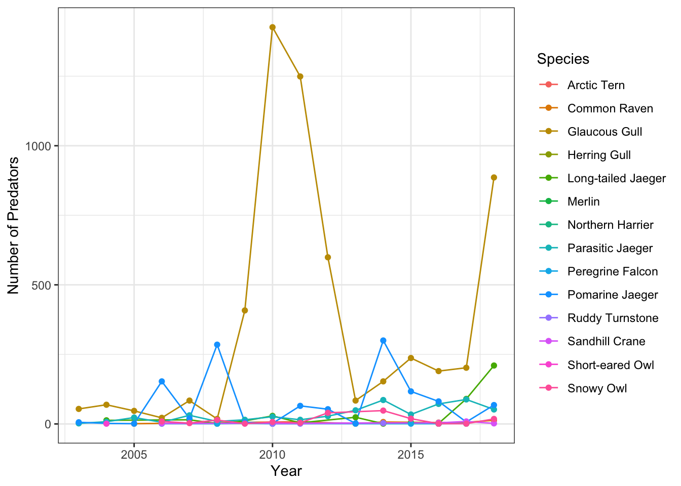
Question 2: Does the number of eggs predated increase with the total number of predators for all species laying nests?
Calculate the number of eggs predated by year and species. Species with no common name were examined, and found to have missing values in the species code as well. This is likely a data entry error that should be examined more closely, but for simplicity here we can drop these rows.
nests_species <- assign_species_name(nests, species) %>%
  group_by(common_name, year) %>%
  summarise(total_predated = sum(number_eggs_predated, na.rm = T),
            .groups = "drop") %>%
  filter(!is.na(common_name))
## Warning in assign_species_name(nests, species): Common
## name has 4 rows containing NACalculate total number of predators across all species by year.
pred_total <- pred_species %>%
    group_by(year) %>%
    summarise(pred_count = sum(pred_count, na.rm = T), .groups = "drop")
Join egg predation data to total predator data.
Plot the number of eggs predated by total predators, faceted over species.
ggplot(nest_pred, aes(x = pred_count, y = total_predated)) +
    geom_point() +
    facet_wrap(~common_name, scales = "free_y", ncol = 2) +
    labs(x = "Number of Predators", y = "Number of Eggs Predated") +
    theme_bw()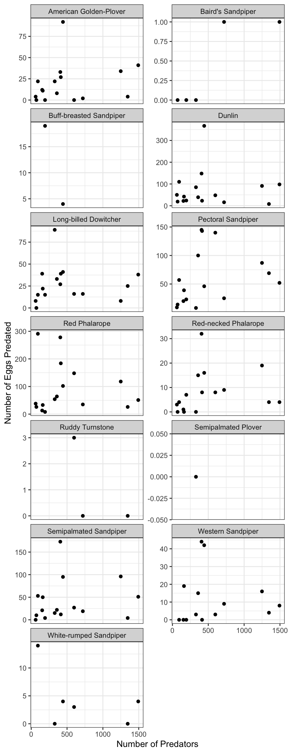
5.15 Spatial vector analysis using sf
5.15.1 Learning Objectives
In this lesson, you will learn:
- How to use the
sfpackage to analyze geospatial data - Static mapping with ggplot
- interactive mapping with
leaflet
5.15.2 Introduction
From the sf vignette:
Simple features or simple feature access refers to a formal standard (ISO 19125-1:2004) that describes how objects in the real world can be represented in computers, with emphasis on the spatial geometry of these objects. It also describes how such objects can be stored in and retrieved from databases, and which geometrical operations should be defined for them.
The sf package is an R implementation of Simple Features. This package incorporates:
- a new spatial data class system in R
- functions for reading and writing data
- tools for spatial operations on vectors
Most of the functions in this package starts with prefix st_ which stands for spatial and temporal.
In this tutorial, our goal is to use a shapefile of Alaska regions and data on population in Alaska by community to create a map that looks like this:
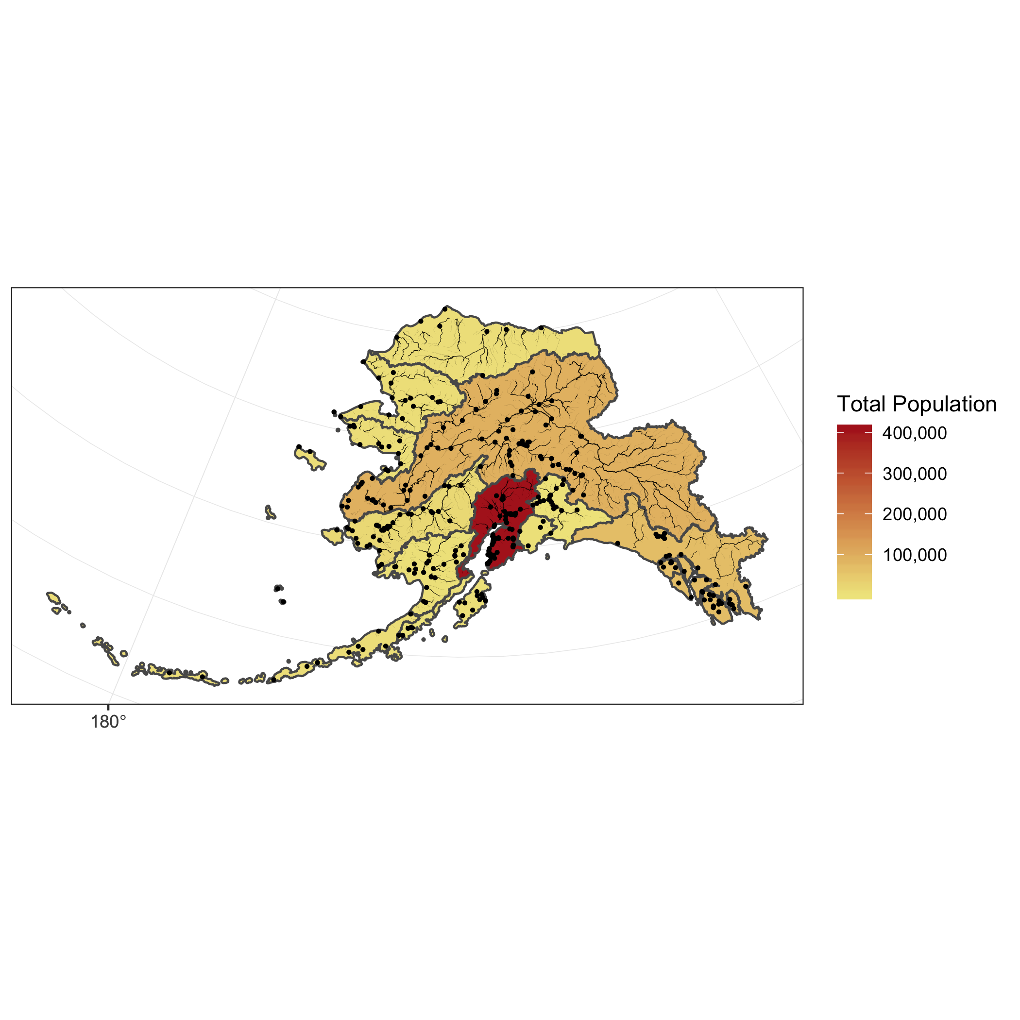
The data we will be using to create the map are:
- Alaska regional boundaries
- Community locations and population
- Alaksa rivers
5.15.3 Working with geospatial data
All of the data used in this tutorial are simplified versions of real datasets available on the KNB. I’ve simplified the original high-resolution geospatial datasets to ease the processing burden on your computers while learning how to do the analysis. These simplified versions of the datasets may contain topological errors. The original version of the datasets are indicated throughout the chapter.
Setup
For convience, I’ve hosted a zipped copy of all of the files on our test site.
Follow these steps to get ready for the next exercise:
- Navigate to this dataset and download the zip folder.
- Create a new folder in your training_username project called “shapefiles”
- Click the “upload” button on RStudio server, and upload the file to the shapefiles directory
- Open your .gititnore file and add that directory to the list of things to ignore.
- Save and commit the changes to your .gitignore.
The first file we will use is a shapefile of regional boundaries in alaska derived from: Jared Kibele and Jeanette Clark. 2018. State of Alaska’s Salmon and People Regional Boundaries. Knowledge Network for Biocomplexity. doi:10.5063/F1125QWP.
Now we can load the libraries we need:
Read in the data and look at a plot of it.
## Read in shapefile using sf
ak_regions <- read_sf("shapefiles/ak_regions_simp.shp")

plot(ak_regions) 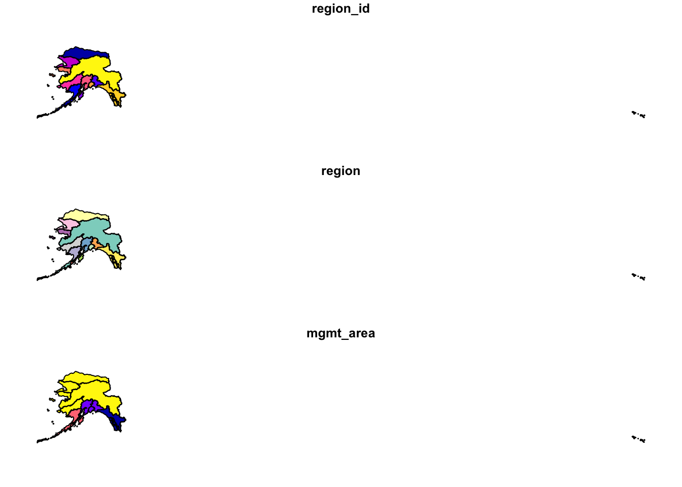
We can also examine it’s class.
## [1] "sf" "tbl_df" "tbl" "data.frame"sf objects usually have two types - sf and data.frame. Two main differences comparing to a regular data.frame object are spatial metadata (geometry type, dimension, bbox, epsg (SRID), proj4string) and additional column - typically named geometry.
Since our shapefile object has the data.frame class, viewing the contents of the object using the head function shows similar results to data we read in using read.csv.
## Simple feature collection with 6 features and 3 fields
## geometry type:  MULTIPOLYGON
## dimension:      XY
## bbox:           xmin: -179.2296 ymin: 51.15702 xmax: 179.8567 ymax: 71.43957
## CRS:            4326
## # A tibble: 6 x 4
##   region_id region  mgmt_area                  geometry
##       <int> <chr>       <dbl>        <MULTIPOLYGON [°]>
## 1         1 Aleuti…         3 (((-171.1345 52.44974, -…
## 2         2 Arctic          4 (((-139.9552 68.70597, -…
## 3         3 Bristo…         3 (((-159.8745 58.62778, -…
## 4         4 Chignik         3 (((-155.8282 55.84638, -…
## 5         5 Copper…         2 (((-143.8874 59.93931, -…
## 6         6 Kodiak          3 (((-151.9997 58.83077, -…
Coordinate Reference System
Every sf object needs a coordinate reference system (or crs) defined in order to work with it correctly. A coordinate reference system contains both a datum and a projection. The datum is how you georeference your points (in 3 dimensions!) onto a spheroid. The projection is how these points are mathematically transformed to represent the georeferenced point on a flat piece of paper. All coordinate reference systems require a datum. However, some coordinate reference systems are “unprojected” (also called geographic coordinate systems). Coordinates in latitude/longitude use a geographic (unprojected) coordinate system. One of the most commonly used geographic coordinate systems is WGS 1984.
ESRI has a blog post that explains these concepts in more detail with very helpful diagrams and examples.
You can view what crs is set by using the function st_crs
## Coordinate Reference System:
##   User input: 4326
##   wkt:
## GEOGCS["WGS 84",
##     DATUM["WGS_1984",
##         SPHEROID["WGS 84",6378137,298.257223563,
##             AUTHORITY["EPSG","7030"]],
##         AUTHORITY["EPSG","6326"]],
##     PRIMEM["Greenwich",0,
##         AUTHORITY["EPSG","8901"]],
##     UNIT["degree",0.0174532925199433,
##         AUTHORITY["EPSG","9122"]],
##     AUTHORITY["EPSG","4326"]]
This is pretty confusing looking. Without getting into the details, that long string says that this data has a greographic coordinate system (WGS84) with no projection. A convenient way to reference crs quickly is by using the EPSG code, a number that represents a standard projection and datum. You can check out a list of (lots!) of EPSG codes here.
We will use several EPSG codes in this lesson. Here they are, along with their more readable names:
- 3338: Alaska Albers
- 4326: WGS84 (World Geodetic System 1984), used in GPS
- 3857: Pseudo-Mercator, used in Google Maps, OpenStreetMap, Bing, ArcGIS, ESRI
You will often need to transform your geospatial data from one coordinate system to another. The st_transform function does this quickly for us. You may have noticed the maps above looked wonky because of the dateline. We might want to set a different projection for this data so it plots nicer. A good one for Alaska is called the Alaska Albers projection, with an EPSG code of 3338.
## Coordinate Reference System:
##   User input: EPSG:3338
##   wkt:
## PROJCS["NAD83 / Alaska Albers",
##     GEOGCS["NAD83",
##         DATUM["North_American_Datum_1983",
##             SPHEROID["GRS 1980",6378137,298.257222101,
##                 AUTHORITY["EPSG","7019"]],
##             TOWGS84[0,0,0,0,0,0,0],
##             AUTHORITY["EPSG","6269"]],
##         PRIMEM["Greenwich",0,
##             AUTHORITY["EPSG","8901"]],
##         UNIT["degree",0.0174532925199433,
##             AUTHORITY["EPSG","9122"]],
##         AUTHORITY["EPSG","4269"]],
##     PROJECTION["Albers_Conic_Equal_Area"],
##     PARAMETER["standard_parallel_1",55],
##     PARAMETER["standard_parallel_2",65],
##     PARAMETER["latitude_of_center",50],
##     PARAMETER["longitude_of_center",-154],
##     PARAMETER["false_easting",0],
##     PARAMETER["false_northing",0],
##     UNIT["metre",1,
##         AUTHORITY["EPSG","9001"]],
##     AXIS["X",EAST],
##     AXIS["Y",NORTH],
##     AUTHORITY["EPSG","3338"]]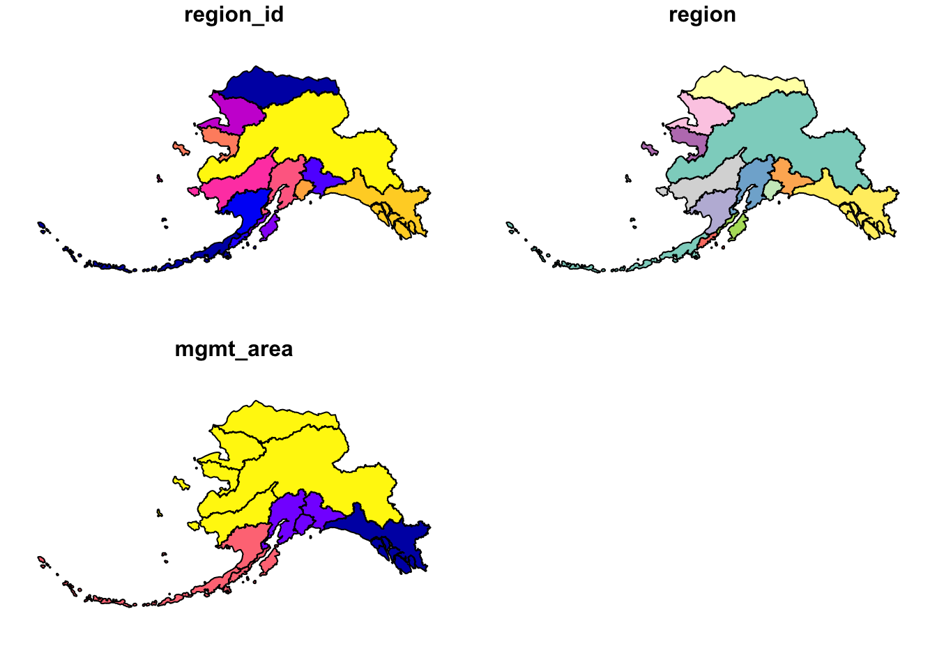
Much better!
5.15.4 sf & the Tidyverse
sf objects can be used as a regular data.frame object in many operations. We already saw the results of plot and head.
Challenge
Try running some other functions you might use to explore a regular data.frame on your sf flavored data.frame.
Since sf objects are data.frames, they play nicely with packages in the tidyverse. Here are a couple of simple examples:
select()
## Simple feature collection with 13 features and 1 field
## geometry type:  MULTIPOLYGON
## dimension:      XY
## bbox:           xmin: -2175328 ymin: 405653.9 xmax: 1579226 ymax: 2383770
## CRS:            EPSG:3338
## # A tibble: 13 x 2
##    region                                      geometry
##    <chr>                             <MULTIPOLYGON [m]>
##  1 Aleutian Isl… (((-1156666 420855.1, -1159837 417990…
##  2 Arctic        (((571289.9 2143072, 569941.5 2142691…
##  3 Bristol Bay   (((-339688.6 973904.9, -339302 972297…
##  4 Chignik       (((-114381.9 649966.8, -112866.8 6520…
##  5 Copper River  (((561012 1148301, 559393.7 1148169, …
##  6 Kodiak        (((115112.5 983293, 113051.3 982825.9…
##  7 Kotzebue      (((-678815.3 1819519, -677555.2 18206…
##  8 Kuskokwim     (((-1030125 1281198, -1029858 1282333…
##  9 Cook Inlet    (((35214.98 1002457, 36660.3 1002038,…
## 10 Norton Sound  (((-848357 1636692, -846510 1635203, …
## 11 Prince Willi… (((426007.1 1087250, 426562.5 1088591…
## 12 Southeast     (((1287777 744574.1, 1290183 745970.8…
## 13 Yukon         (((-375318 1473998, -373723.9 1473487…
Note the sticky geometry column! The geometry column will stay with your sf object even if it is not called explicitly.
filter()
## Simple feature collection with 1 feature and 3 fields
## geometry type:  MULTIPOLYGON
## dimension:      XY
## bbox:           xmin: 559475.7 ymin: 722450 xmax: 1579226 ymax: 1410576
## CRS:            EPSG:3338
## # A tibble: 1 x 4
##   region_id region  mgmt_area                  geometry
## *     <int> <chr>       <dbl>        <MULTIPOLYGON [m]>
## 1        12 Southe…         1 (((1287777 744574.1, 129…
Joins
You can also use the sf package to create spatial joins, useful for when you want to utilize two datasets together. As an example, let’s ask a question: how many people live in each of these Alaska regions?
We have some population data, but it gives the number of people by city, not by region. To determine the number of people per region we will need to:
- read in the city data from a csv and turn it into an
sfobject - use a spatial join (
st_join) to assign each city to a region - use
group_byandsummarizeto calculate the total population by region
First, read in the population data as a regular data.frame. This data is derived from: Jeanette Clark, Sharis Ochs, Derek Strong, and National Historic Geographic Information System. 2018. Languages used in Alaskan households, 1990-2015. Knowledge Network for Biocomplexity. doi:10.5063/F11G0JHX. Unnecessary columns were removed and the most recent year of data was selected.
The st_join function is a spatial left join. The arguments for both the left and right tables are objects of class sf which means we will first need to turn our population data.frame with latitude and longitude coordinates into an sf object.
We can do this easily using the st_as_sf function, which takes as arguments the coordinates and the crs. The remove = F specification here ensures that when we create our geometry column, we retain our original lat lng columns, which we will need later for plotting. Although it isn’t said anywhere explicitly in the file, let’s assume that the coordinate system used to reference the latitude longitude coordinates is WGS84, which has a crs number of 4236.
## Simple feature collection with 6 features and 5 fields
## geometry type:  POINT
## dimension:      XY
## bbox:           xmin: -176.6581 ymin: 51.88 xmax: -154.1703 ymax: 62.68889
## CRS:            EPSG:4326
##   year     city      lat       lng population
## 1 2015     Adak 51.88000 -176.6581        122
## 2 2015   Akhiok 56.94556 -154.1703         84
## 3 2015 Akiachak 60.90944 -161.4314        562
## 4 2015    Akiak 60.91222 -161.2139        399
## 5 2015   Akutan 54.13556 -165.7731        899
## 6 2015 Alakanuk 62.68889 -164.6153        777
##                     geometry
## 1    POINT (-176.6581 51.88)
## 2 POINT (-154.1703 56.94556)
## 3 POINT (-161.4314 60.90944)
## 4 POINT (-161.2139 60.91222)
## 5 POINT (-165.7731 54.13556)
## 6 POINT (-164.6153 62.68889)
Now we can do our spatial join! You can specify what geometry function the join uses (st_intersects, st_within, st_crosses, st_is_within_distance, …) in the join argument. The geometry function you use will depend on what kind of operation you want to do, and the geometries of your shapefiles.
In this case, we want to find what region each city falls within, so we will use st_within.
This gives an error!
Error: st_crs(x) == st_crs(y) is not TRUETurns out, this won’t work right now because our coordinate reference systems are not the same. Luckily, this is easily resolved using st_transform, and projecting our population object into Alaska Albers.
## Simple feature collection with 6 features and 8 fields
## geometry type:  POINT
## dimension:      XY
## bbox:           xmin: -1537925 ymin: 472627.8 xmax: -10340.71 ymax: 1456223
## CRS:            EPSG:3338
##   year     city      lat       lng population
## 1 2015     Adak 51.88000 -176.6581        122
## 2 2015   Akhiok 56.94556 -154.1703         84
## 3 2015 Akiachak 60.90944 -161.4314        562
## 4 2015    Akiak 60.91222 -161.2139        399
## 5 2015   Akutan 54.13556 -165.7731        899
## 6 2015 Alakanuk 62.68889 -164.6153        777
##   region_id           region mgmt_area
## 1         1 Aleutian Islands         3
## 2         6           Kodiak         3
## 3         8        Kuskokwim         4
## 4         8        Kuskokwim         4
## 5         1 Aleutian Islands         3
## 6        13            Yukon         4
##                     geometry
## 1  POINT (-1537925 472627.8)
## 2 POINT (-10340.71 770998.4)
## 3  POINT (-400885.5 1236460)
## 4  POINT (-389165.7 1235475)
## 5 POINT (-766425.7 526057.8)
## 6  POINT (-539724.9 1456223)
Challenge
Like we mentioned above, there are many different types of joins you can do with geospatial data. Examine the help page for these joins (?st_within will get you there). What other joins types might be appropriate for examining the relationship between points and polygyons? What about two sets of polygons?
Group and summarize
Next we compute the total population for each region. In this case, we want to do a group_by and summarise as this were a regular data.frame - otherwise all of our point geometries would be included in the aggreation, which is not what we want. Our goal is just to get the total population by region. We remove the sticky geometry using as.data.frame, on the advice of the sf::tidyverse help page.
pop_region <- pop_joined %>%
  as.data.frame() %>%
  group_by(region) %>%
  summarise(total_pop = sum(population))
## `summarise()` ungrouping output (override with `.groups` argument)## # A tibble: 6 x 2
## region total_pop
## <chr> <int>
## 1 Aleutian Islands 8840
## 2 Arctic 8419
## 3 Bristol Bay 6947
## 4 Chignik 311
## 5 Cook Inlet 408254
## 6 Copper River 2294And use a regular left_join to get the information back to the Alaska region shapefile. Note that we need this step in order to regain our region geometries so that we can make some maps.
## Joining, by = "region"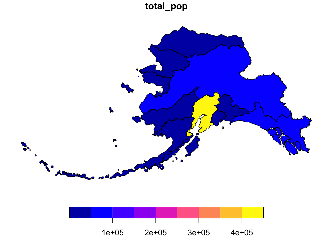
So far, we have learned how to use sf and dplyr to use a spatial join on two datasets and calculate a summary metric from the result of that join.
The group_by and summarize functions can also be used on sf objects to summarize within a dataset and combine geometries. Many of the tidyverse functions have methods specific for sf objects, some of which have additional arguments that wouldn’t be relevant to the data.frame methods. You can run ?sf::tidyverse to get documentation on the tidyverse sf methods.
Let’s try some out. Say we want to calculate the population by Alaska management area, as opposed to region.
## `summarise()` ungrouping output (override with `.groups` argument)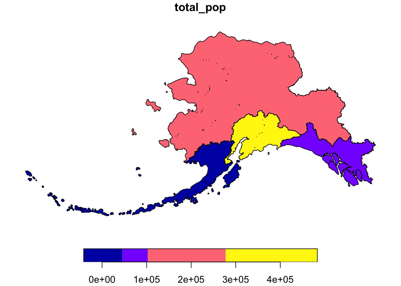
Notice that the region geometries were combined into a single polygon for each management area.
If we don’t want to combine geometries, we can specify do_union = F as an argument.
pop_mgmt_3338 <- pop_region_3338 %>%
  group_by(mgmt_area) %>%
  summarize(total_pop = sum(total_pop), do_union = F)
## `summarise()` ungrouping output (override with `.groups` argument)
Writing the file
Save the spatial object to disk using write_sf() and specifying the filename. Writing your file with the extension .shp will assume an ESRI driver driver, but there are many other format options available.
5.15.5 Visualize with ggplot
ggplot2 now has integrated functionality to plot sf objects using geom_sf().
We can plot sf objects just like regular data.frames using geom_sf.
ggplot(pop_region_3338) +
  geom_sf(aes(fill = total_pop)) +
  theme_bw() +
  labs(fill = "Total Population") +
  scale_fill_continuous(low = "khaki", high =  "firebrick", labels = comma)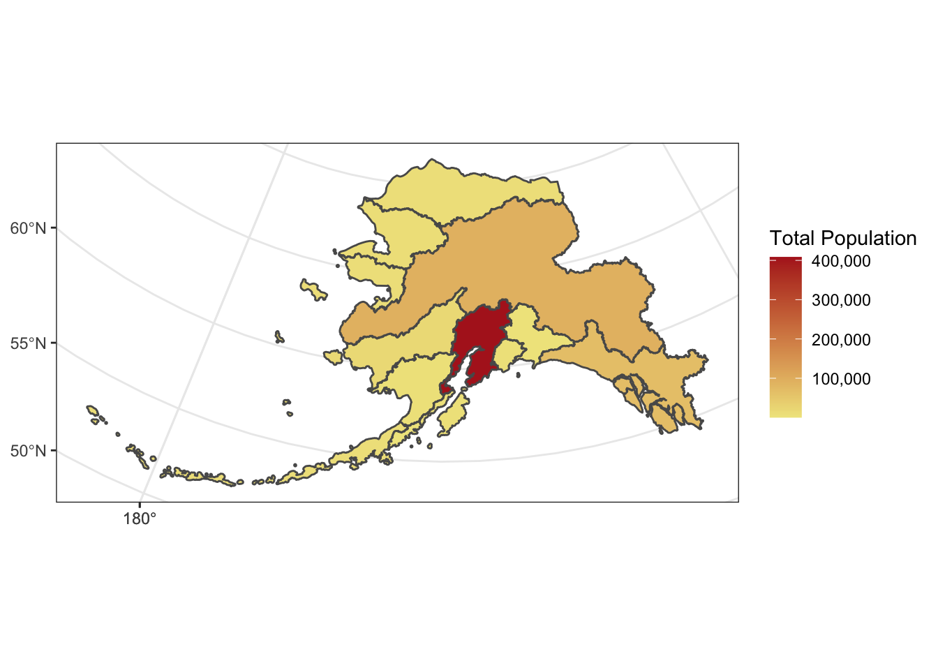
We can also plot multiple shapefiles in the same plot. Say if we want to visualize rivers in Alaska, in addition to the location of communities, since many communities in Alaska are on rivers. We can read in a rivers shapefile, doublecheck the crs to make sure it is what we need, and then plot all three shapefiles - the regional population (polygons), the locations of cities (points), and the rivers (linestrings).
The rivers shapefile is a simplified version of Jared Kibele and Jeanette Clark. Rivers of Alaska grouped by SASAP region, 2018. Knowledge Network for Biocomplexity. doi:10.5063/F1SJ1HVW.
## Coordinate Reference System:
##   No user input
##   wkt:
## PROJCS["Albers",
##     GEOGCS["GCS_GRS 1980(IUGG, 1980)",
##         DATUM["unknown",
##             SPHEROID["GRS80",6378137,298.257222101]],
##         PRIMEM["Greenwich",0],
##         UNIT["Degree",0.017453292519943295]],
##     PROJECTION["Albers_Conic_Equal_Area"],
##     PARAMETER["standard_parallel_1",55],
##     PARAMETER["standard_parallel_2",65],
##     PARAMETER["latitude_of_center",50],
##     PARAMETER["longitude_of_center",-154],
##     PARAMETER["false_easting",0],
##     PARAMETER["false_northing",0],
##     UNIT["Meter",1]]
Note that although no EPSG code is set explicitly, with some sluething we can determine that this is EPSG:3338. This site is helpful for looking up EPSG codes.
ggplot() +
  geom_sf(data = pop_region_3338, aes(fill = total_pop)) +
  geom_sf(data = rivers_3338, aes(size = StrOrder), color = "black") +
  geom_sf(data = pop_3338, aes(), size = .5) +
  scale_size(range = c(0.01, 0.2), guide = F) +
  theme_bw() +
  labs(fill = "Total Population") +
  scale_fill_continuous(low = "khaki", high =  "firebrick", labels = comma)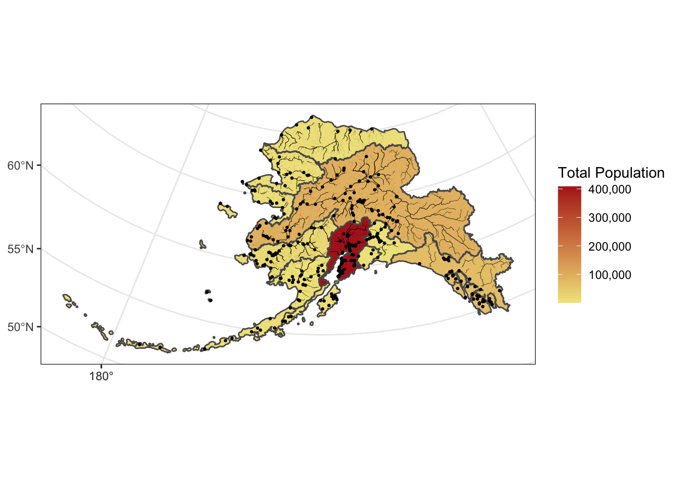
Incorporate base maps into static maps using ggmap
The ggmap package has some functions that can render base maps (as raster objects) from open tile servers like Google Maps, Stamen, OpenStreetMap, and others.
We’ll need to transform our shapefile with population data by community to EPSG:3857 which is the CRS used for rendering maps in Google Maps, Stamen, and OpenStreetMap, among others.
Next, let’s grab a base map from the Stamen map tile server covering the region of interest.
First we include a function that transforms the bounding box (which starts in EPSG:4326) to also be in the EPSG:3857 CRS, which is the projection that the map raster is returned in from Stamen. This is an issue with ggmap described in more detail here
# Define a function to fix the bbox to be in EPSG:3857
# See https://github.com/dkahle/ggmap/issues/160#issuecomment-397055208
ggmap_bbox_to_3857 <- function(map) {
  if (!inherits(map, "ggmap")) stop("map must be a ggmap object")
  # Extract the bounding box (in lat/lon) from the ggmap to a numeric vector,
  # and set the names to what sf::st_bbox expects:
  map_bbox <- setNames(unlist(attr(map, "bb")),
                       c("ymin", "xmin", "ymax", "xmax"))

  # Coonvert the bbox to an sf polygon, transform it to 3857,
  # and convert back to a bbox (convoluted, but it works)
  bbox_3857 <- st_bbox(st_transform(st_as_sfc(st_bbox(map_bbox, crs = 4326)), 3857))

  # Overwrite the bbox of the ggmap object with the transformed coordinates
  attr(map, "bb")$ll.lat <- bbox_3857["ymin"]
  attr(map, "bb")$ll.lon <- bbox_3857["xmin"]
  attr(map, "bb")$ur.lat <- bbox_3857["ymax"]
  attr(map, "bb")$ur.lon <- bbox_3857["xmax"]
  map
}
Next, we define the bounding box of interest, and use get_stamenmap() to get the basemap. Then we run our function defined above on the result of the get_stamenmap() call.
bbox <- c(-170, 52, -130, 64)   # This is roughly southern Alaska
ak_map <- get_stamenmap(bbox, zoom = 4)
ak_map_3857 <- ggmap_bbox_to_3857(ak_map)
Finally, plot both the base raster map with the population data overlayed, which is easy now that everything is in the same projection (3857):
ggmap(ak_map_3857) +
  geom_sf(data = pop_3857, aes(color = population), inherit.aes = F) +
  scale_color_continuous(low = "khaki", high =  "firebrick", labels = comma)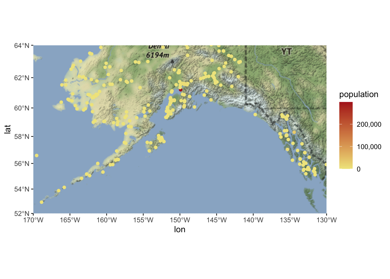
5.15.6 Visualize sf objects with leaflet
We can also make an interactive map from our data above using leaflet.
Leaflet (unlike ggplot) will project data for you. The catch is that you have to give it both a projection (like Alaska Albers), and that your shapefile must use a geographic coordinate system. This means that we need to use our shapefile with the 4326 EPSG code. Remember you can always check what crs you have set using st_crs.
Here we define a leaflet projection for Alaska Albers, and save it as a variable to use later.
epsg3338 <- leaflet::leafletCRS(
  crsClass = "L.Proj.CRS",
  code = "EPSG:3338",
  proj4def =  "+proj=aea +lat_1=55 +lat_2=65 +lat_0=50 +lon_0=-154 +x_0=0 +y_0=0 +ellps=GRS80 +towgs84=0,0,0,0,0,0,0 +units=m +no_defs",
  resolutions = 2^(16:7))
You might notice that this looks familiar! The syntax is a bit different, but most of this information is also contained within the crs of our shapefile:
## Coordinate Reference System:
##   User input: EPSG:3338
##   wkt:
## PROJCS["NAD83 / Alaska Albers",
##     GEOGCS["NAD83",
##         DATUM["North_American_Datum_1983",
##             SPHEROID["GRS 1980",6378137,298.257222101,
##                 AUTHORITY["EPSG","7019"]],
##             TOWGS84[0,0,0,0,0,0,0],
##             AUTHORITY["EPSG","6269"]],
##         PRIMEM["Greenwich",0,
##             AUTHORITY["EPSG","8901"]],
##         UNIT["degree",0.0174532925199433,
##             AUTHORITY["EPSG","9122"]],
##         AUTHORITY["EPSG","4269"]],
##     PROJECTION["Albers_Conic_Equal_Area"],
##     PARAMETER["standard_parallel_1",55],
##     PARAMETER["standard_parallel_2",65],
##     PARAMETER["latitude_of_center",50],
##     PARAMETER["longitude_of_center",-154],
##     PARAMETER["false_easting",0],
##     PARAMETER["false_northing",0],
##     UNIT["metre",1,
##         AUTHORITY["EPSG","9001"]],
##     AXIS["X",EAST],
##     AXIS["Y",NORTH],
##     AUTHORITY["EPSG","3338"]]
Since leaflet requires that we use an unprojected coordinate system, let’s use st_transform yet again to get back to WGS84.
m <- leaflet(options = leafletOptions(crs = epsg3338)) %>%
        addPolygons(data = pop_region_4326,
                    fillColor = "gray",
                    weight = 1)

m
We can add labels, legends, and a color scale.
pal <- colorNumeric(palette = "Reds", domain = pop_region_4326$total_pop)

m <- leaflet(options = leafletOptions(crs = epsg3338)) %>%
        addPolygons(data = pop_region_4326,
                    fillColor = ~pal(total_pop),
                    weight = 1,
                    color = "black",
                    fillOpacity = 1,
                    label = ~region) %>%
        addLegend(position = "bottomleft",
                  pal = pal,
                  values = range(pop_region_4326$total_pop),
                  title = "Total Population")

m
We can also add the individual communities, with popup labels showing their population, on top of that!
pal <- colorNumeric(palette = "Reds", domain = pop_region_4326$total_pop)

m <- leaflet(options = leafletOptions(crs = epsg3338)) %>%
        addPolygons(data = pop_region_4326,
                    fillColor = ~pal(total_pop),
                    weight = 1,
                    color = "black",
                    fillOpacity = 1) %>%
        addCircleMarkers(data = pop_4326,
                         lat = ~lat,
                         lng = ~lng,
                         radius = ~log(population/500), # arbitrary scaling
                         fillColor = "gray",
                         fillOpacity = 1,
                         weight = 0.25,
                         color = "black",
                         label = ~paste0(pop_4326$city, ", population ", comma(pop_4326$population))) %>%
        addLegend(position = "bottomleft",
                  pal = pal,
                  values = range(pop_region_4326$total_pop),
                  title = "Total Population")

m
There is a lot more functionality to sf including the ability to intersect polygons, calculate distance, create a buffer, and more. Here are some more great resources and tutorials for a deeper dive into this great package:
Raster analysis in R
Spatial analysis in R with the sf package
Intro to Spatial Analysis
sf github repo
Tidy spatial data in R: using dplyr, tidyr, and ggplot2 with sf
mapping-fall-foliage-with-sf
5.16 DataONE Data Portals
DataONE is a federated network of data repositories, including NEON, that enables search and discovery of Earth and environmental science data from a single location. With over 1M data records spanning multiple domains, there is undoubtedly a significant amount of data that may not be relevant to a particular research network, collaboration or question. Data portals allow for the creation and display of subsets or ‘collections’ of data from within the DataONE network, each with their own search capabilities, portal level documentation and metrics. In this way, researchers can easily view project information and datasets from across the federated network of repositories all in one place.
In this unit we describe the main features of data portals and step researchers through the process of creating a data portal for the first time. As an individual researcher you may choose to use data portals to showcase your data objects that have been published across multiple repositories. However, they can also be used to create a custom collection of data from within a single repository, such as NEON.
5.16.1 What is a Portal?
A portal is a collection of DataONE federated repository data packages on a unique webpage.
Typically, a research project’s website won’t be maintained beyond the life of the project and all the information on the website that provides context for the data collection is lost. Portals can provide a means to preserve information regarding the projects’ objectives, scopes, and organization and couple this with the data files so it’s clear how to use and interpret the data for years to come. Plus, when datasets are scattered across the repositories in the DataONE network, portals can help see them all in one convenient webpage.
Portals also leverage DataONE’s metric features, which create statistics describing the project’s data packages. Information such as total size of data, proportion of data file types, and data collection periods are immediately available from the portal webpage.
5.16.2 Portal Uses
Portals allow users to bundle supplementary information about their group, data, or project along with the data packages. Data contributors can organize their project specific data packages into a unique portal and customize the portal’s theme and structure according to the needs of that project.
Researchers can also use portals to compare their public data packages and highlight and share them with other teams, as well as the broader research audience.
To see an example of what portals could look like, please view the Toolik Field Station’s portal.
5.16.3 Portal Main Components
Portals have five components: an about page, a settings page, a data page, a metrics page, and customizable free-form pages.
5.16.3.1 About Page
This page is the first page users will see after initially creating a new portal, and it is highly recommended that users use this feature to create a description for their portal. Add a picture of your logo, a title and description of your portal, and freeform text using the markdown editor.
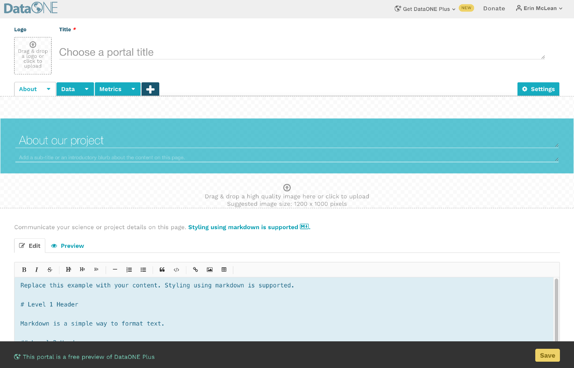
5.16.3.2 Settings Tab
On the settings tab, users can give the portal a title and assign it a unique url; also referred to as a portal identifier. Users can add a general description of the portal, upload an icon photo for their data, and upload icon photos from any partner organizations that have contributed to the data. These partner icons will appear in the footer banner on every page in a portal, likewise your portal icon will appear in the header banner.
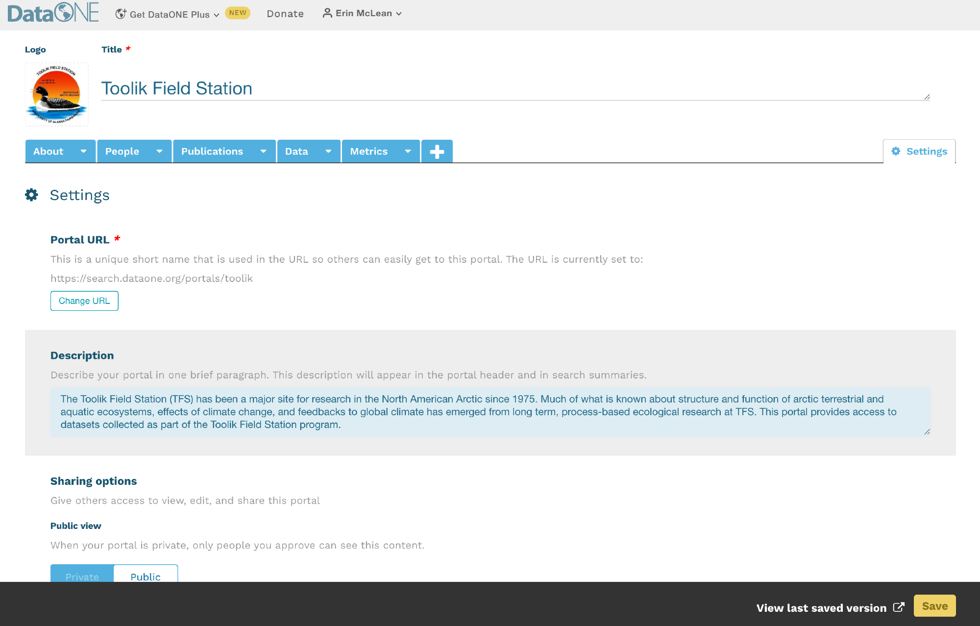
Every DataONE portal URL will follow this format:
https://search.dataone.org/portals/portal_identifier
5.16.3.3 Data Page
The data page is the most important component of the DataONE portal system. This is where users will display the data packages of their choice. It looks and performs just like the main DataONE user interface.
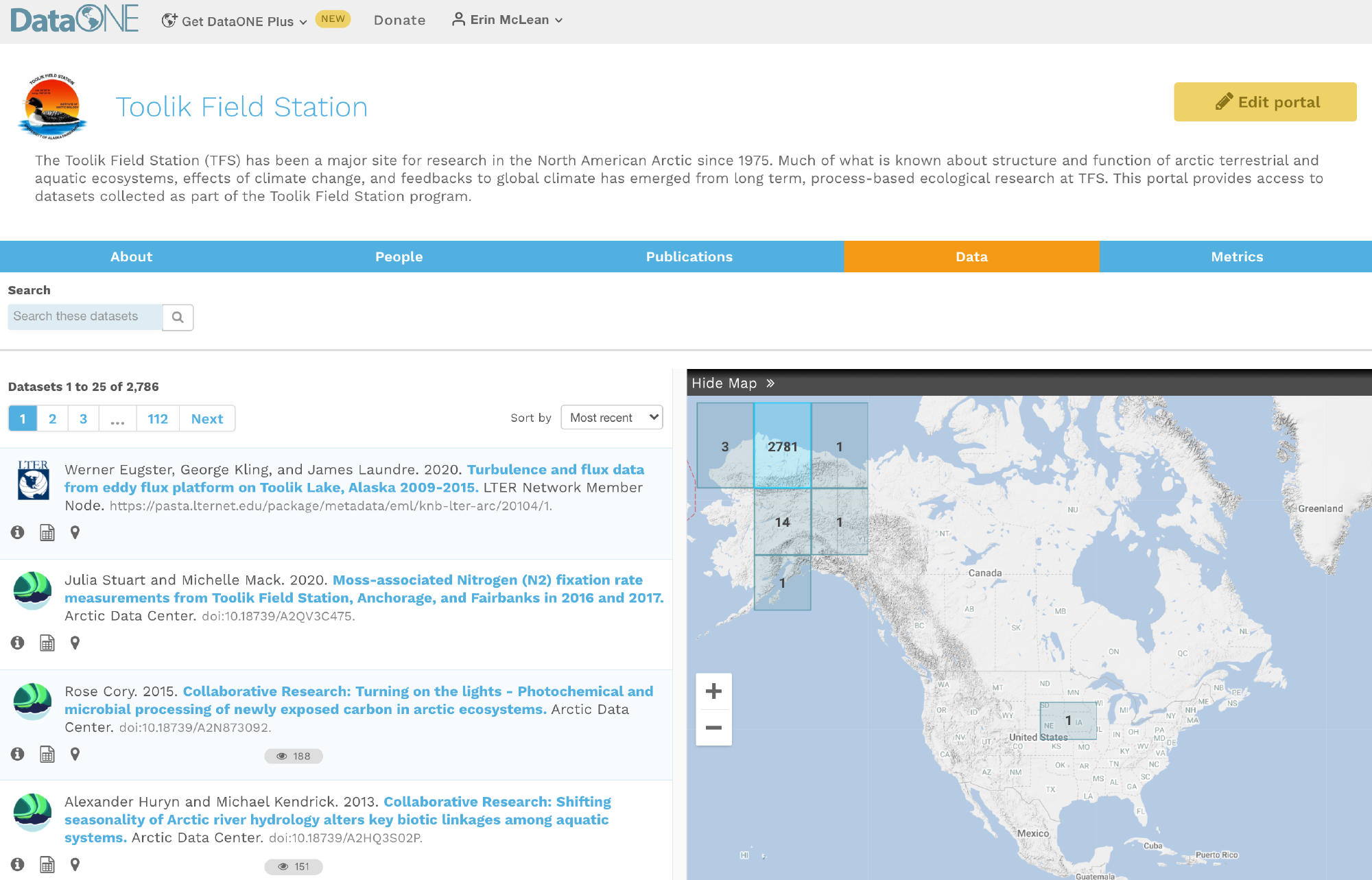
5.16.3.4 Metrics Page
Unlike the first two pages, the metrics page cannot be edited or customized. It is a default feature that provides the following information about the data packages within a portal:
- The total number of publicly-available metadata records
- The volume (in bytes) of all publicly-available metadata records and data files
- The most recent date the datasets were last updated (metadata and data are treated separately)
- The file types of all publicly-available data
- The years in which data was collected, regardless of upload date
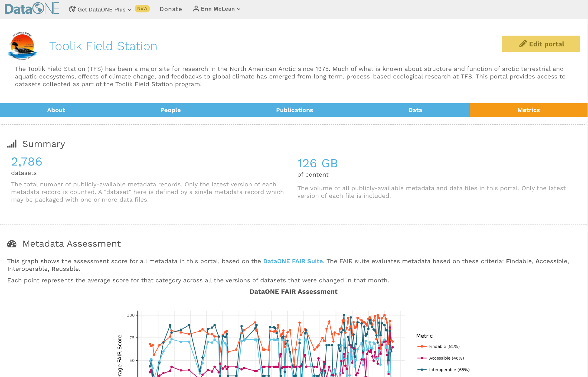
Please contact DataONE’s support team at support@dataone.org about any questions or concerns about the metrics page.
5.16.3.5 Freeform Pages
Freeform pages are an optional function provided by DataONE portals. Here, users can add as much supplementary information as needed using markdown.
5.16.3.5.1 Example Freeform Pages
Below are two examples of ways users can take advantage of portal freeform pages to tie unique content together with their data packages. Users can add as many tabs as needed.
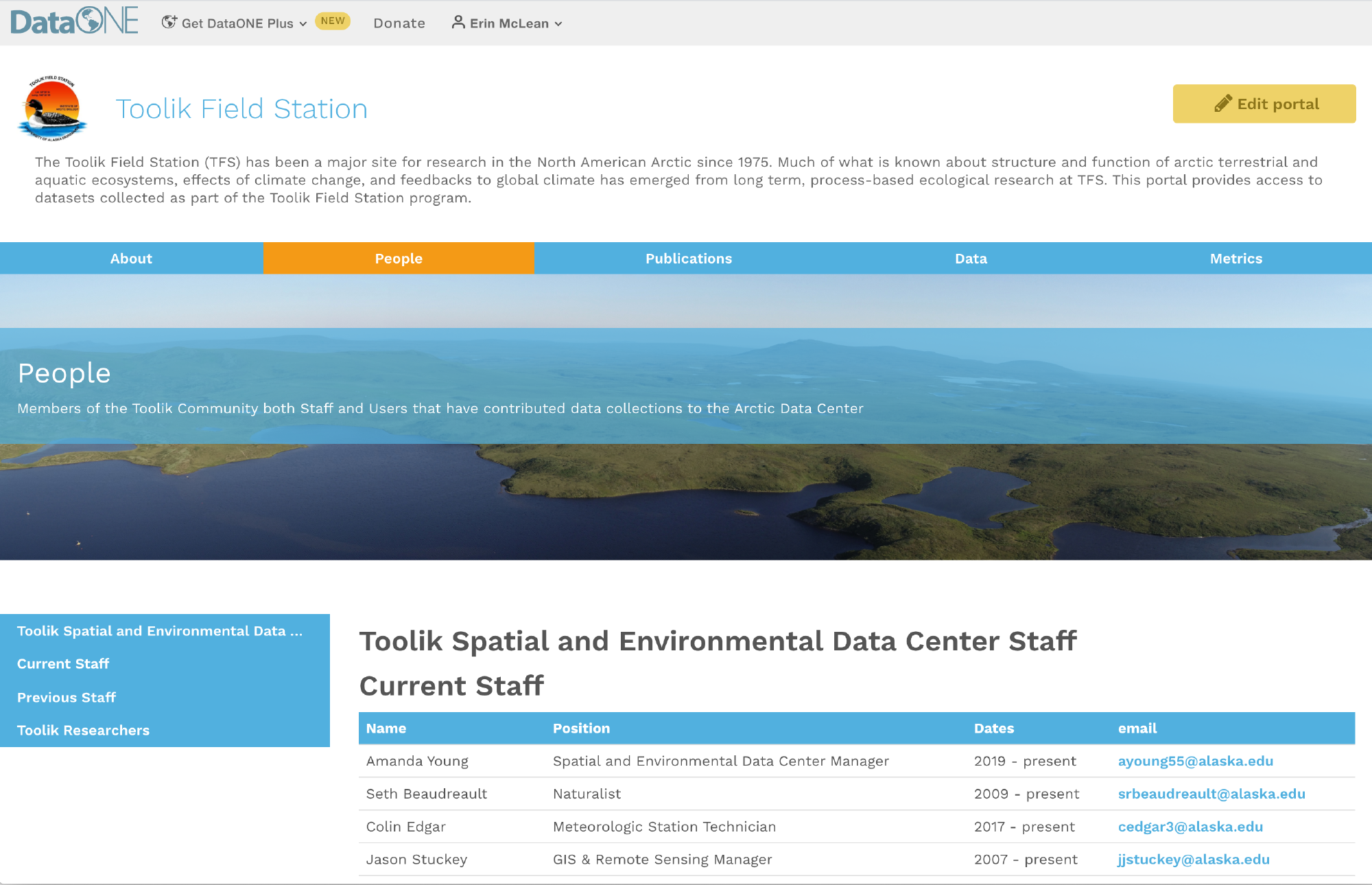
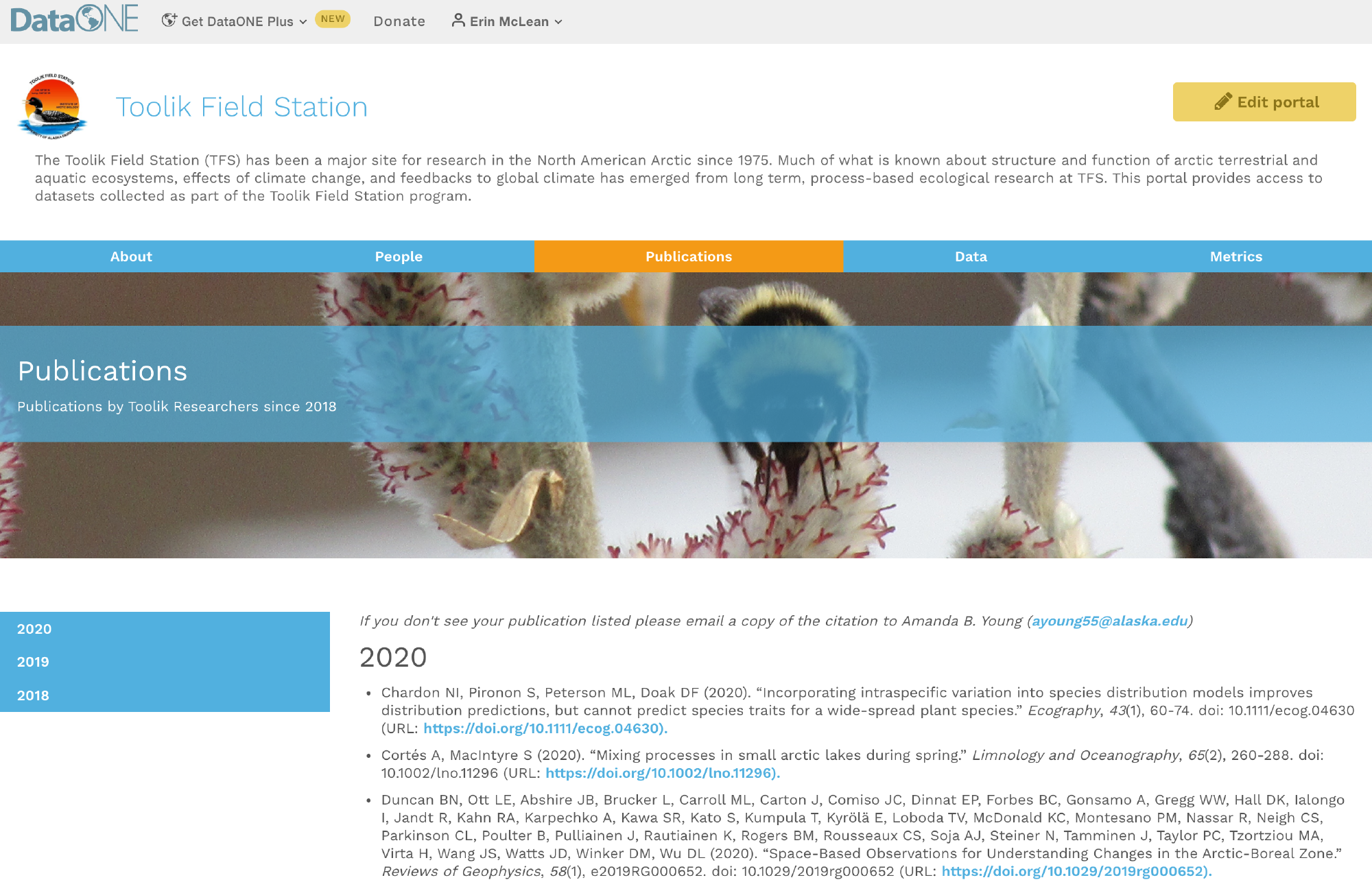
The examples shown on this page are from the Toolik Field Station’s portal; visit this portal to explore its contents further.
5.16.4 Creating Portals
A step-by-step guide on how to navigate DataONE and create a new portal.
Video tutorials on how to create your first portal from the Arctic Data Center, a repository within the DataONE network.
5.16.4.1 Getting Started with Portals
If you are on DataONE’s primary website, click on your name in the upper right hand corner when you are signed in to DataONE with your ORCID. A dropdown will appear, and you would select “My Portals”.

On your profile settings page, select ‘My Portals’. After the page loads select the yellow button ‘+ New Portal’ to add a new portal, you’ll automatically be directed to a fresh edit session.
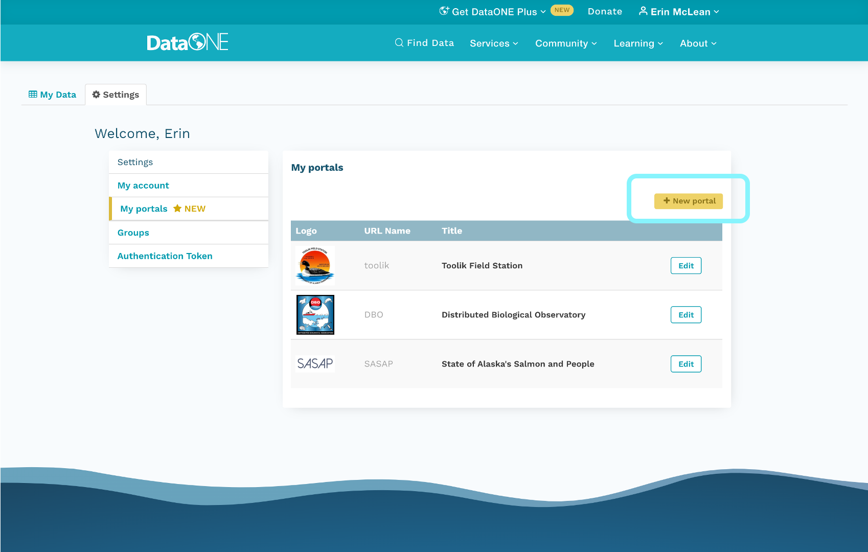
5.16.4.2 Portal About and Settings Page
In a new edit session, the first thing you’ll see is the about page where you’ll be able to add details about your project page.
On the settings tab, you’ll set the basic elements of your portal:
Portal title
Unique portal identifier
- This identifier will be used to create the portal URL. If the name is available, a label will indicate it’s available and if the name is taken already, it will note that the name is already taken. This feature ensures the portals are unique.
Portal description
Partner organization logos
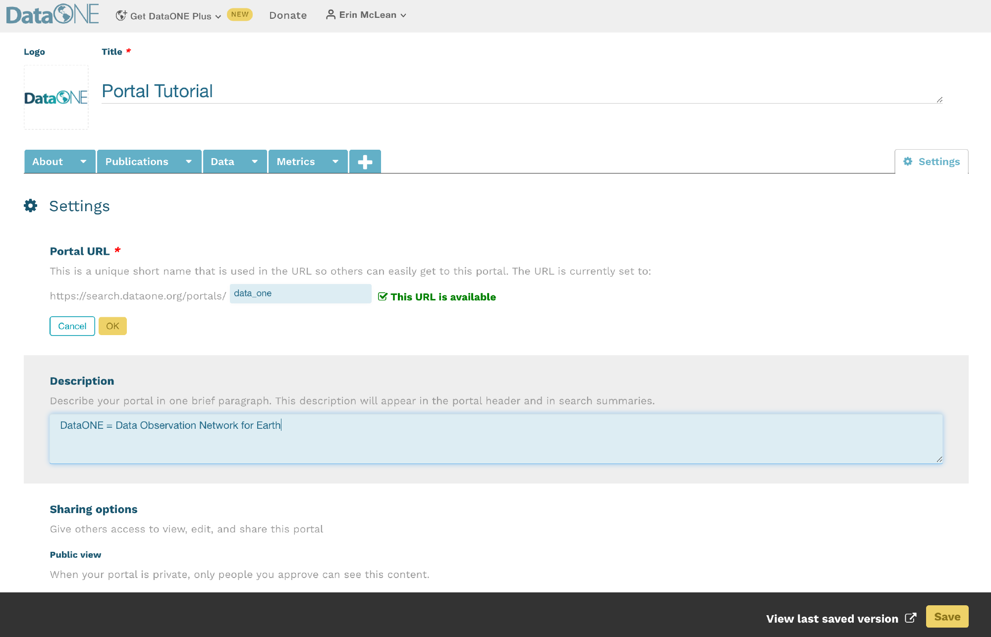
Adding collaborators to help you create your portal is as straightforward as copying and pasting in their ORCID into the box below the permissions section. You can choose whether the collaborator can view, edit, or is an owner of the portal. You can have multiples of each role.
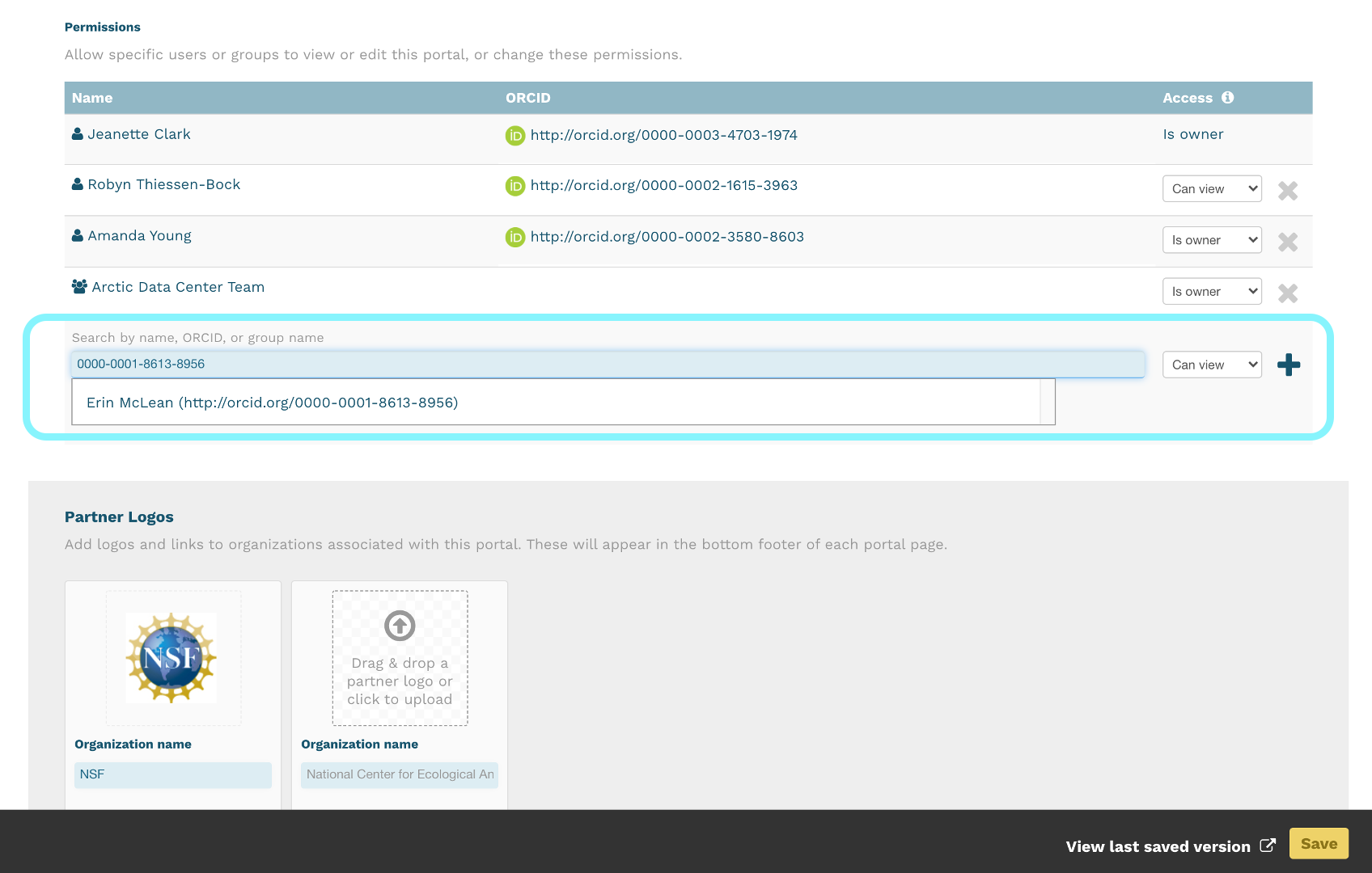
5.16.5 Adding Data to Portals
Video tutorials on using portal search filters from the Arctic Data Center
Navigate to the ‘Data’ tab. Here you will see a list of all the datasets across the DataONE network. In order to populate a portal with the data packages applicable to your needs, narrow the search results using the filters on the left side of the page. When you’ve selected the data you want, hit the yellow save button in the bottom right.
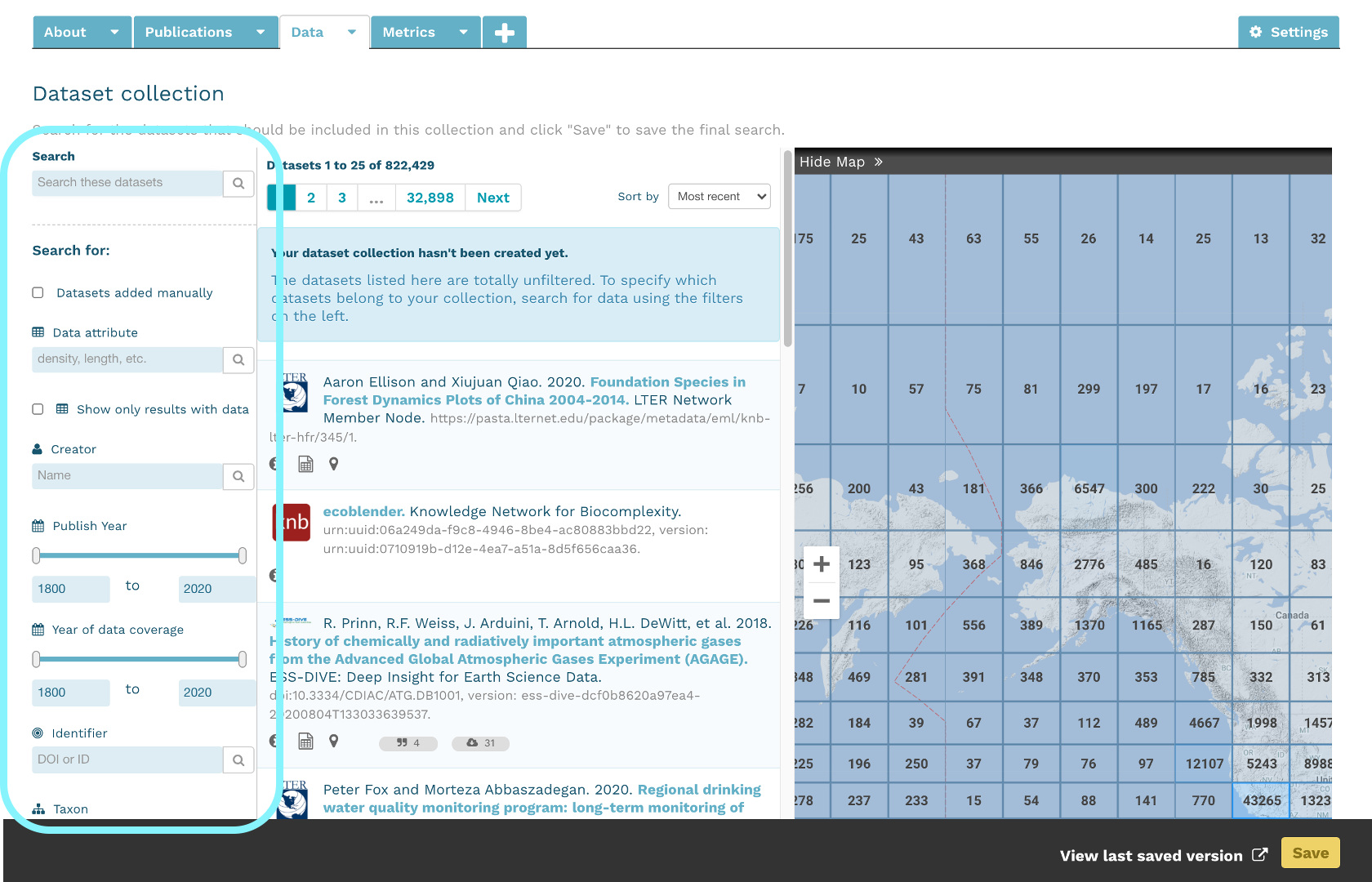
The portal search feature has the following filters available:
- Search: A general search feature that will return data packages with the entered term in the package metadata
- Creator: We recommend searching by last names for more accurate results.
- Publish Year: Use either the sliding scale or enter start and end years manually
- Year of Data Coverage: Searches for data packages with temporal coverages within the selected date range. As with the Publish Year search, use either the sliding scale or enter manually
- Identifier: Searches for all or part of the DOI (digital object identifier) associated with the dataset
- Taxon: Searches for any taxonomic rank specified by the submitter
- Location: This filter will search within the data packages’ geographic description field, meaning that you can search by both name or type of location (eg. United States or forest)
If you need assistance assembling portal data using a complex query, please contact the DataONE Support Team.
5.16.5.1 Data Package Metrics
As stated in Portal Main Components, the metrics page is a default function provided by DataONE. This page cannot be edited and cannot be viewed while editing. Users do have the option to delete the page if they’d like. To delete the page, select the arrow next to the word “Metrics” in the tab and choose “Delete” from the dropdown list.
To see metric summaries, navigate to your portal in view mode. See Saving and Editing Portals for more information on how to view portals.
Please contact the DataONE Support Team about any questions or concerns about the metrics page.
5.16.6 Creating Unique Freeform Pages
Video tutorials on creating freeform pages from the Arctic Data Center
To add a freeform page to a portal, select the ‘+’ tab next to the data and metric tabs and then choose the freeform option that appears on screen. A freeform page will then populate.
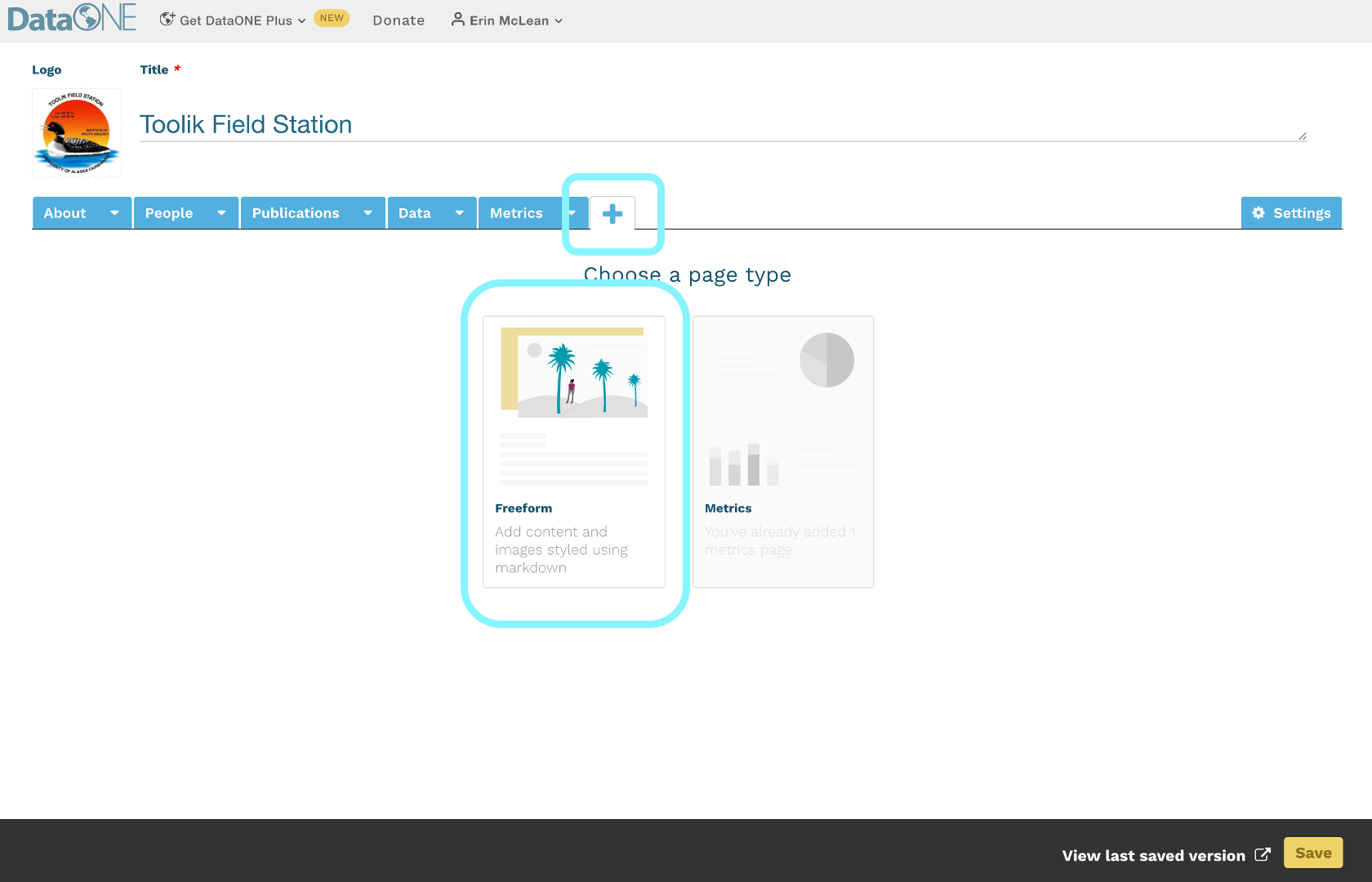
Easily customize your banner with a unique image, title, and page description. To change the name of the tab, click on the arrow in the ‘Untitled’ tab and select ‘Rename’ from the dropdown list.
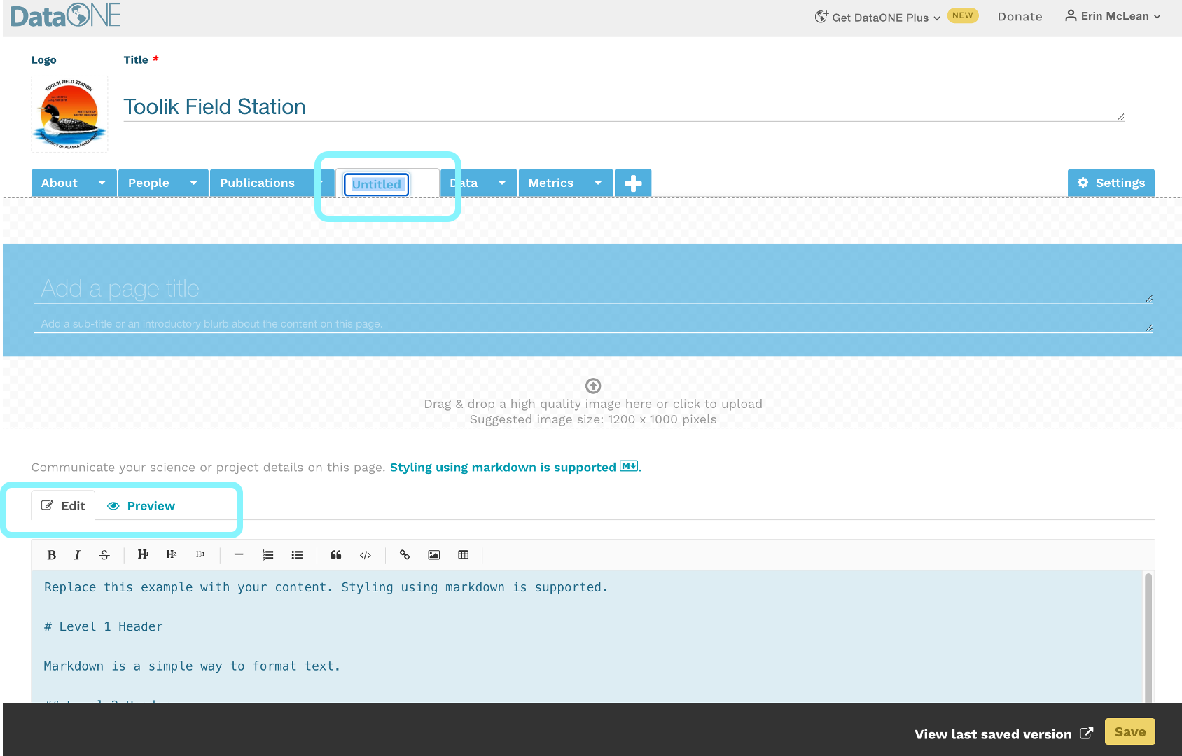
Below the banner, there is a markdown text box with some examples on how to use the markdown formatting directives to customize the text display. There is also a formatting header at the top to assist if you’re unfamiliar with markdown. As you write, toggle through the Edit and Preview modes in the markdown text box to make sure your information is displaying as intended. Portals are flexible and can accommodate as many additional freeform pages as needed.
The markdown header structure helps to generate the table of contents for the page.
Please see these additional resources for help with markdown:
- Markdown reference
- Ten minute tutorial
- For a longer example where you can also preview the results, checkout the Showdown Live Editor
5.16.7 Saving and Editing Portals
Be sure to save your portal when you complete a page to ensure your progress is retained.
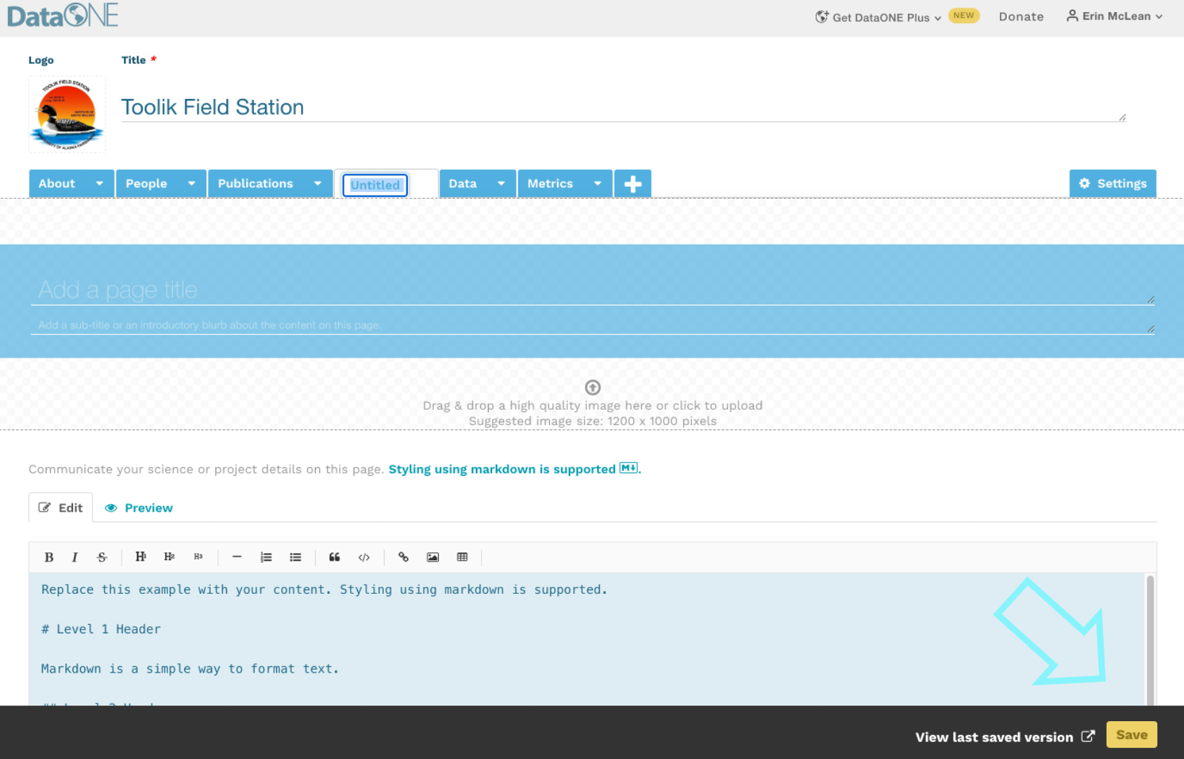
Whenever a portal is saved, a dialogue box will pop up at the top of the page prompting users to view their private portal in view mode. You can choose to ignore this and continue editing.
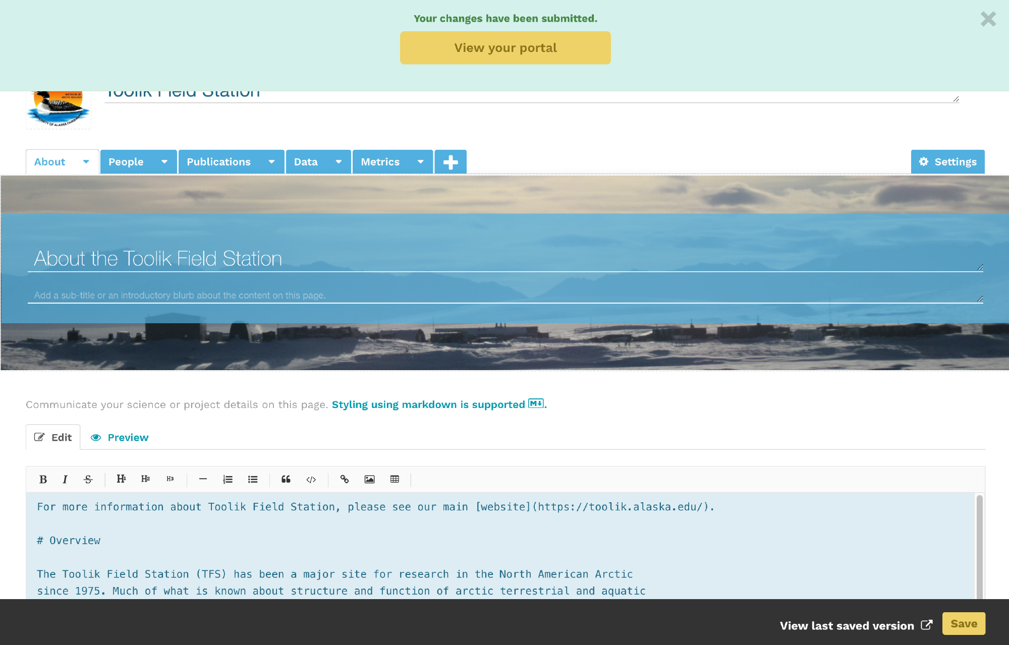
To delete a page from your portal, select the arrow in the tab and choose ‘Delete’ from the dropdown.
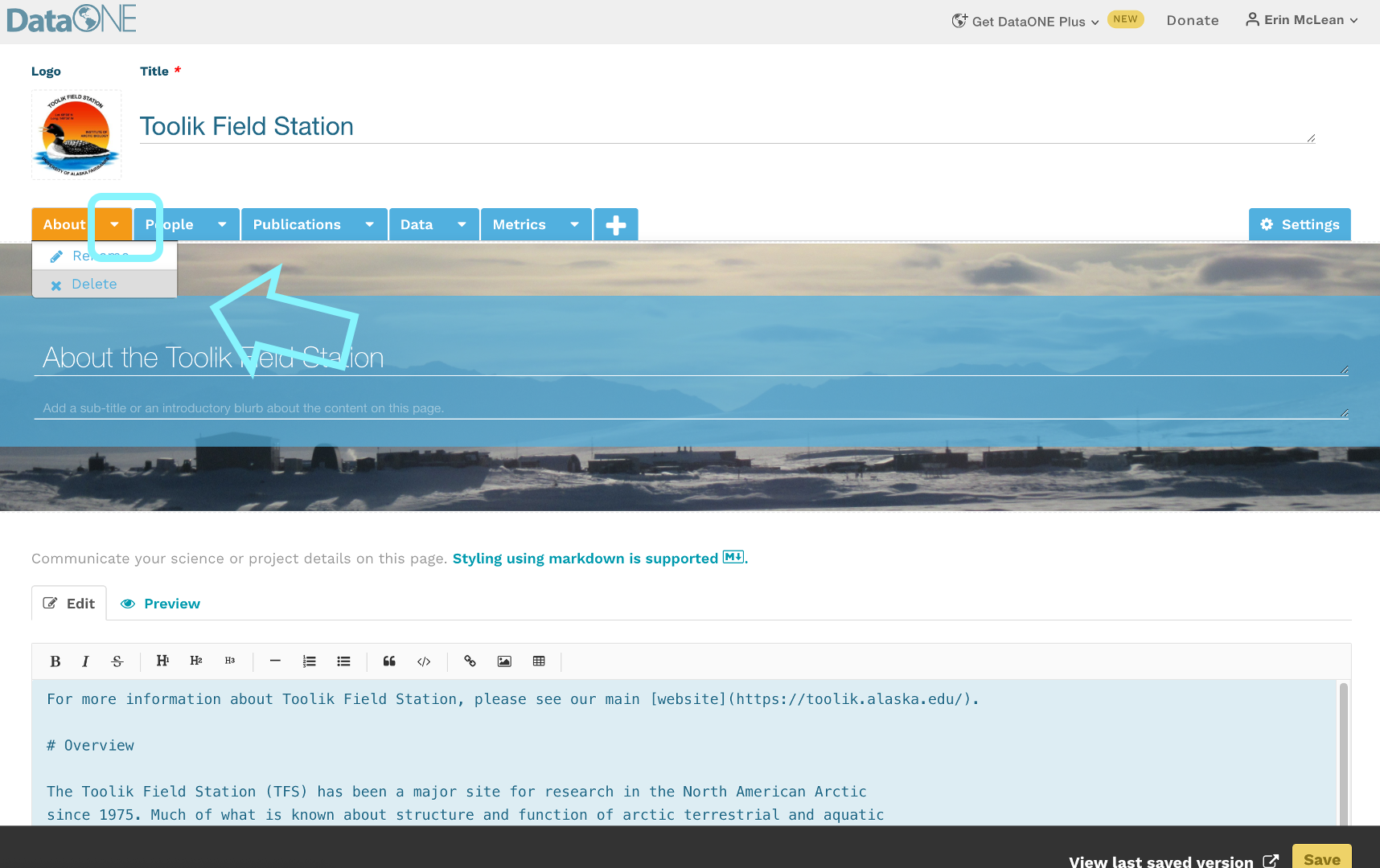
Users can view and edit their portal from their ‘My Portals’ tab.
First, click the arrow your name in the top-right corner to drop down your menu options. Then, select ‘My Portals’ from the dropdown underneath your name. See the section on Getting Started with Portals for more details.
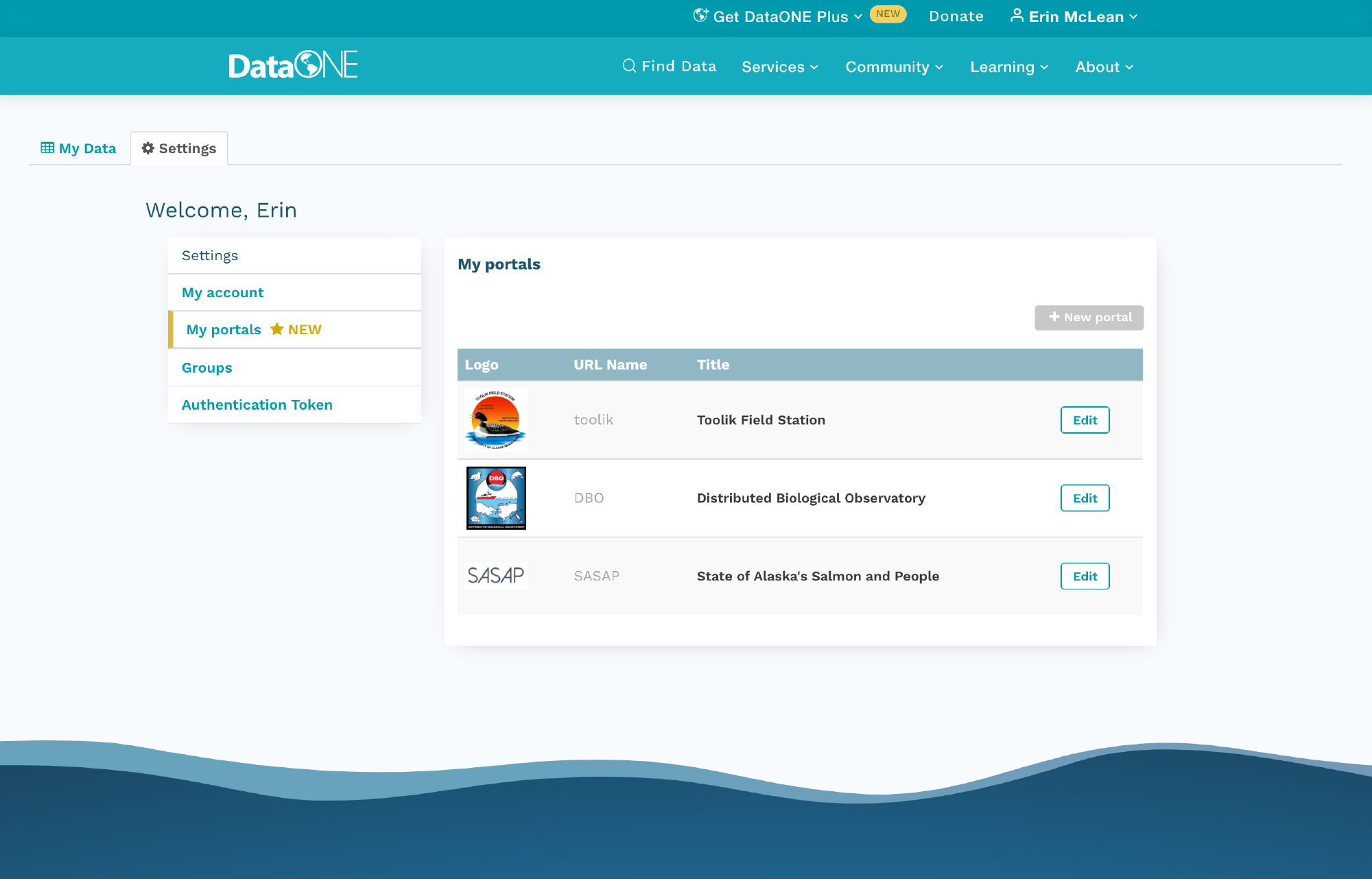
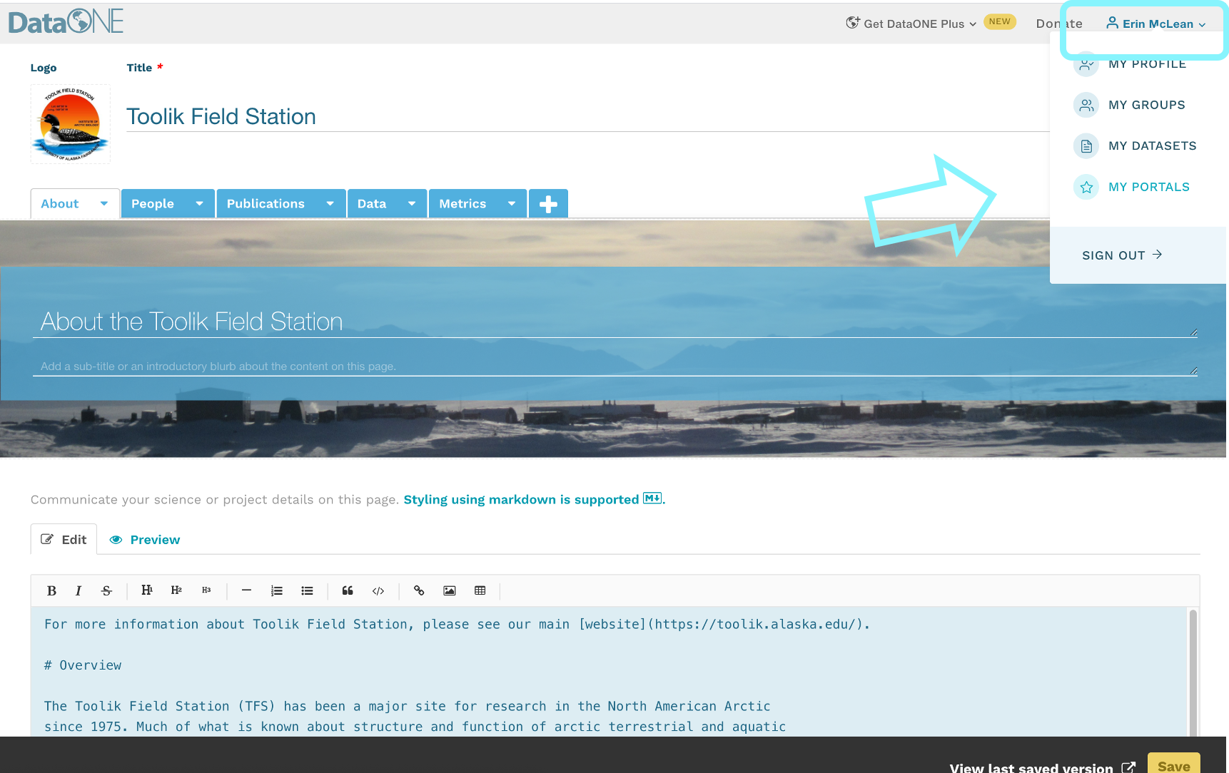
Click on the portal title to view it or select the edit button to make changes.
5.16.8 How to Publish Portals
New portals are automatically set to private and only visible to the portal creator. The portal will remain private until the owner decides to make it public.
To make your portal public, go into the settings of your portal. Under the description, you’ll see a new section called ‘Sharing Options’. You can toggle between your portal being private and your portal being public there.
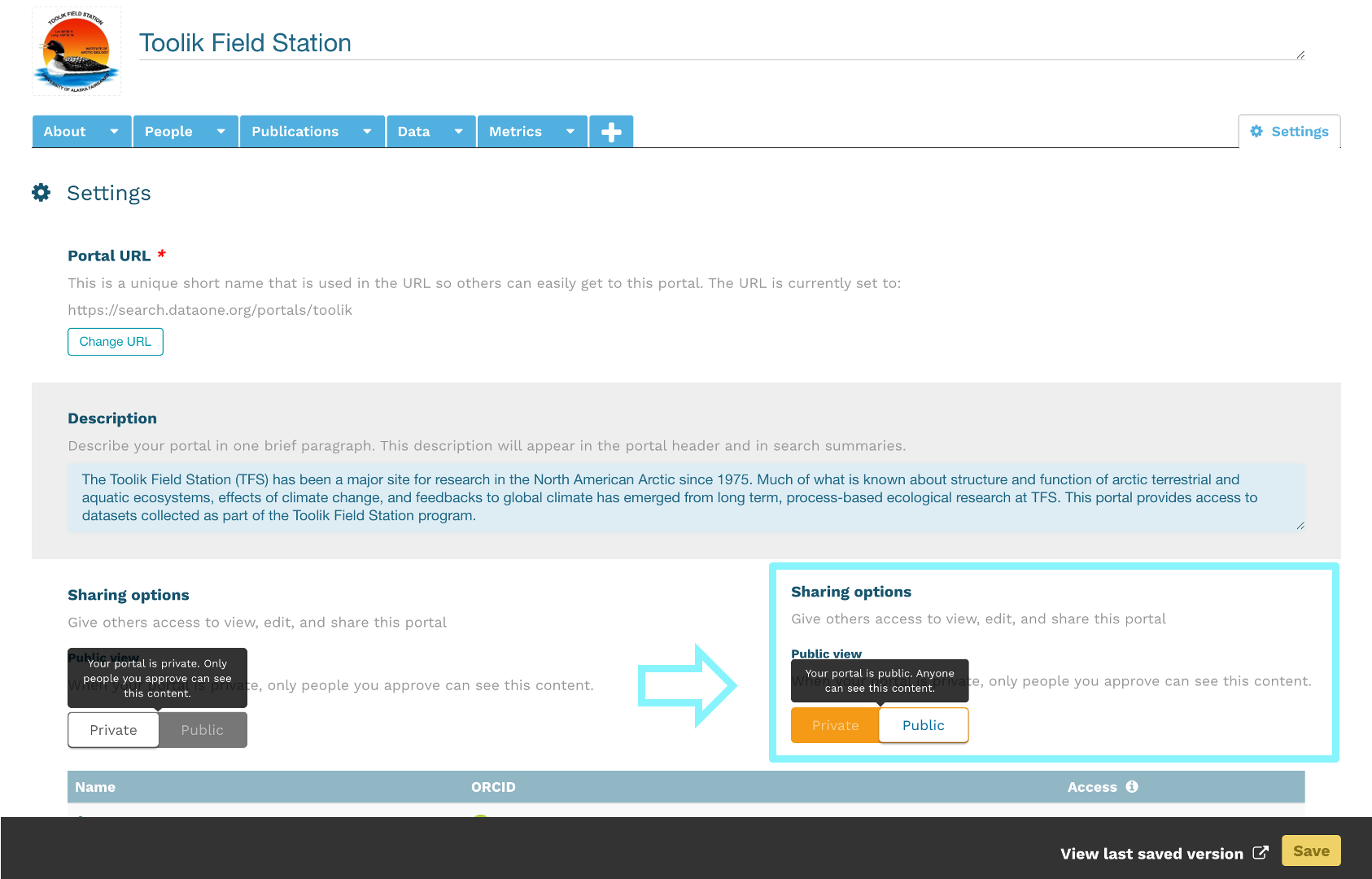
5.16.9 Sharing Portals
In order to share a published portal, users can simply direct recipients to their unique identifier. Portal identifiers are embedded into DataONE’s portal URL: https://search.dataone.org/portals/portal-identifier
To view or edit your portal identifier, go into edit mode in your portal. In the settings page, your portal URL will be the first item on the page.
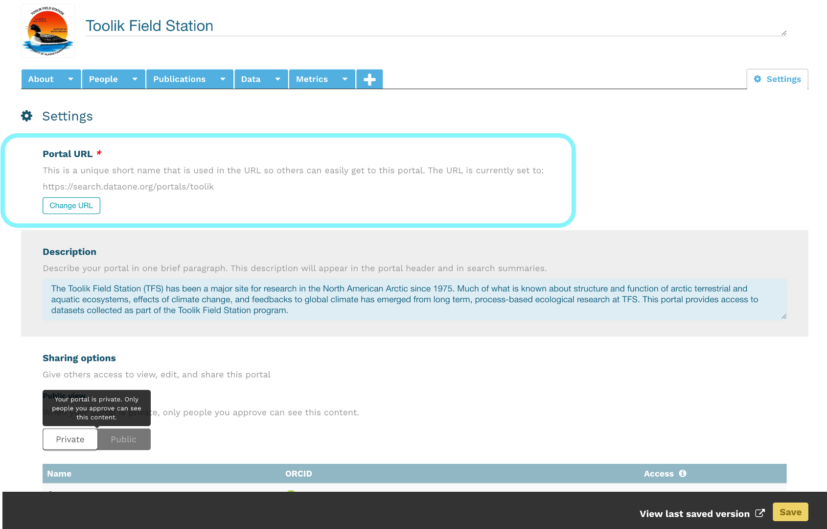
5.16.10 Tutorial Videos
For video tutorials on how to create your first portal visit resources on the Arctic Data Center video tutorial page.
5.16.11 Acknowledgements
Much of this documentation was composed by ESS-DIVE, which can be found here.
5.17 Reproducibility and Provenance
5.17.1 Learning Objectives
In this lesson, you will:
- Learn how to build a reproducible paper in RMarkdown
- Review the importance of computational reproducibility
- Review the of provenance metadata
- Review tools and techniques for reproducibility supported by the NCEAS and DataONE
5.17.1.1 Reproducible Papers
A great overview of this approach to reproducible papers comes from:
Ben Marwick, Carl Boettiger & Lincoln Mullen (2018) Packaging Data Analytical Work Reproducibly Using R (and Friends), The American Statistician, 72:1, 80-88, doi:10.1080/00031305.2017.1375986
This lesson will draw from existing materials:
The key idea in Marwick et al. (2018) is that of the “research compendium”: A single container for not just the journal article associated with your research but also the underlying analysis, data, and even the required software environment required to reproduce your work. Research compendia make it easy for researchers to do their work but also for others to inspect or even reproduce the work because all necessary materials are readily at hand due to being kept in one place. Rather than a constrained set of rules, the research compendium is a scaffold upon which to conduct reproducible research using open science tools such as:
Fortunately for us, Ben Marwick (and others) have written an R package called rrtools that helps us create a research compendium from scratch.
To start a reproducible paper with rrtools, run:
You should see output similar to the below:
> rrtools::use_compendium("mypaper")
The directory mypaper has been created.
✓ Setting active project to '/Users/bryce/mypaper'
✓ Creating 'R/'
✓ Writing 'DESCRIPTION'
Package: mypaper
Title: What the Package Does (One Line, Title Case)
Version: 0.0.0.9000
Authors@R (parsed):
    * First Last <first.last@example.com> [aut, cre]
Description: What the package does (one paragraph).
License: MIT + file LICENSE
ByteCompile: true
Encoding: UTF-8
LazyData: true
Roxygen: list(markdown = TRUE)
RoxygenNote: 7.1.1
✓ Writing 'NAMESPACE'
✓ Writing 'mypaper.Rproj'
✓ Adding '.Rproj.user' to '.gitignore'
✓ Adding '^mypaper\\.Rproj$', '^\\.Rproj\\.user$' to '.Rbuildignore'
✓ Setting active project to '<no active project>'
✓ The package mypaper has been created
✓ Now opening the new compendium...
✓ Done. The working directory is currently /Users/bryce

Next, you need to:  ↓ ↓ ↓
● Edit the DESCRIPTION file
● Use other 'rrtools' functions to add components to the compendium
rrtools has created the beginnings of a research compendium for us.
At this point, it looks mostly the same as an R package.
That’s because it uses the same underlying folder structure and metadata and therefore it technically is an R package.
And this means our research compendium will be easy to install, just like an R package.
Before we get to writing our reproducible paper, let’s fill in some more structure. Let’s:
- Add a license (always a good idea)
- Set up a README file in the RMarkdown format
- Create an
analysisfolder to hold our reproducible paper
usethis::use_apl2_license(name="Your Name") # Change this
rrtools::use_readme_rmd()
rrtools::use_analysis()
At this point, we’re ready to start writing the paper.
To follow the structure rrtools has put in place for us, here are some pointers:
- Edit
./analysis/paper/paper.Rmdto begin writing your paper and your analysis in the same document - Add any citations to
./analysis/paper/references.bib - Add any longer R scripts that don’t fit in your paper in an
Rfolder at the top level - Add raw data to
./data/raw_data - Write out any derived data (generated in
paper.Rmd) to./data/derived_data - Write out any figures in
./analysis/figures
It would also be a good idea to initialize this folder as a git repo for maximum reproducibility:
After that, push a copy up to GitHub.
Hopefully, now that you’ve created a research compendium with rrtools, you can imagine how a pre-defined structure like the one rrtools creates might help you organize your reproducible research and also make it easier for others to understand your work.
For a more complete example than the one we built above, take a look at benmarwick/teaching-replication-in-archaeology.
5.17.1.2 Reproducibility and Provenance
Reproducible Research: Recap
Working in a reproducible manner:
- increases research efficiency, accelerating the pace of your research and collaborations
- provides transparency by capturing and communicating scientific workflows
- enables research to stand on the shoulders of giants (build on work that came before)
- allows credit for secondary usage and supports easy attribution
- increases trust in science
To enable others to fully interpret, reproduce or build upon our research, we need to provide more comprehensive information than is typically included in a figure or publication.
What data were used in this study? What methods applied? What were the parameter settings? What documentation or code are available to us to evaluate the results? Can we trust these data and methods?
Are the results reproducible?
Computational reproducibility is the ability to document data, analyses, and models sufficiently for other researchers to be able to understand and ideally re-execute the computations that led to scientific results and conclusions.
Practically speaking, reproducibility includes:
- Preserving the data
- Preserving the software workflow
- Documenting what you did
- Describing how to interpret it all
Computational Provenance
Computational provenance refers to the origin and processing history of data including:
- Input data
- Workflow/scripts
- Output data
- Figures
- Methods, dataflow, and dependencies
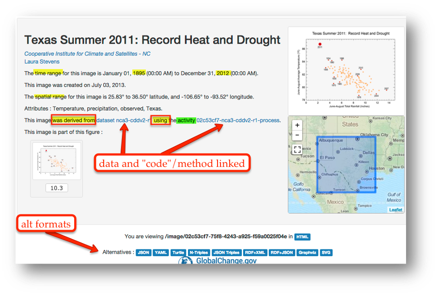
From Provenance to Reproducibility
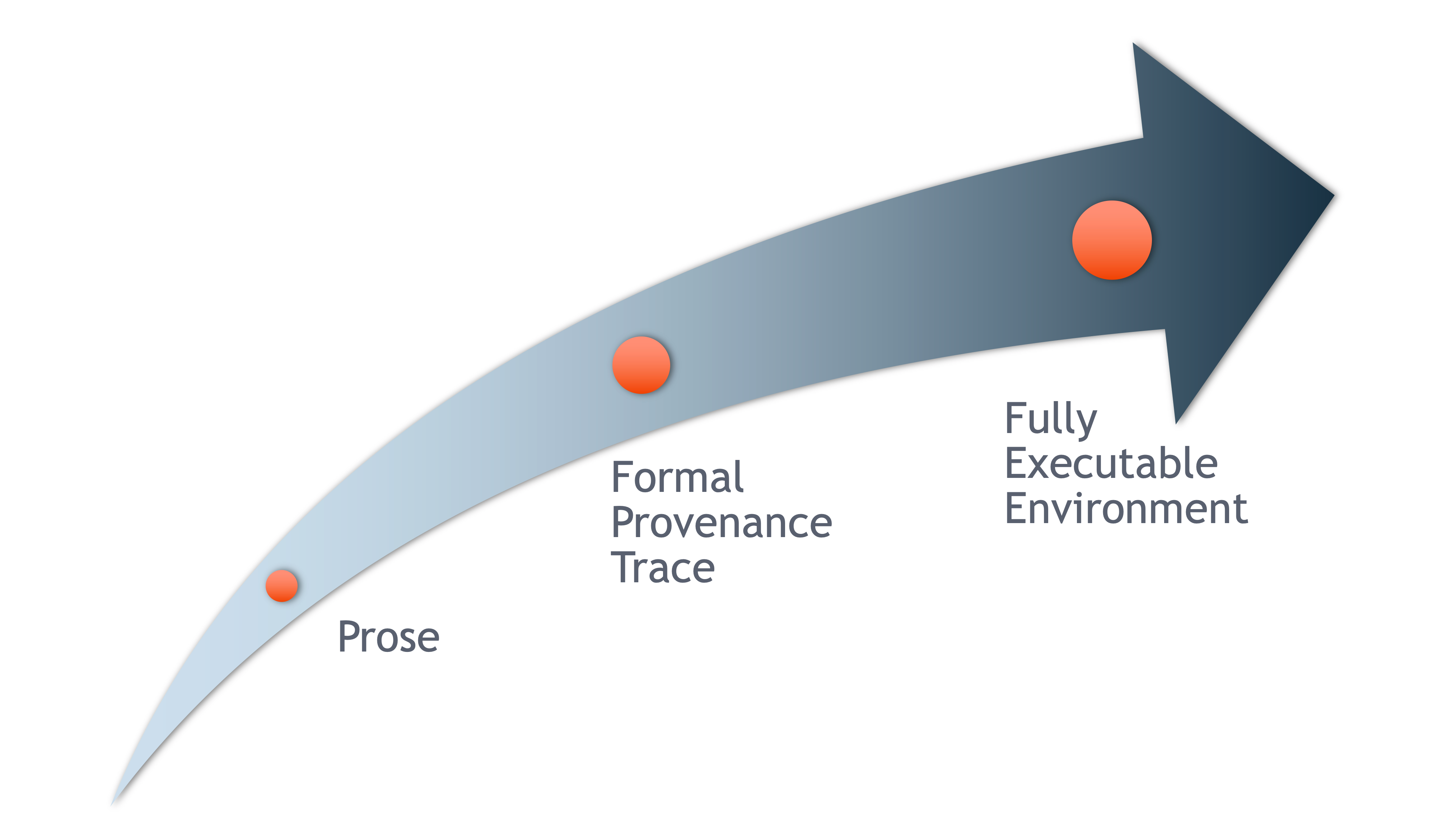
At DataONE we facilitate reproducible science through provenance by:
- Tracking data derivation history
- Tracking data inputs and outputs of analyses
- Tracking analysis and model executions
- Preserving and documenting software workflows
- Linking all of these to publications
Introducing Prov-ONE, an extension of W3C PROV
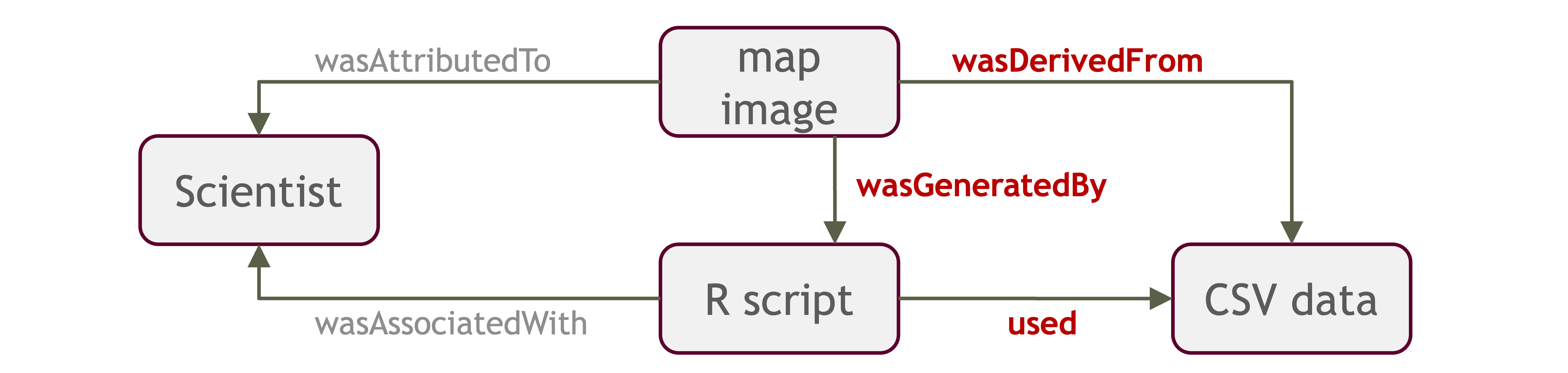
ProvONE provides the fundamental information required to understand and analyze scientific workflow-based computational experiments. It covers the main aspects that have been identified as relevant in the provenance literature including data structure. This addresses the most relevant aspects of how the data, both used and produced by a computational process, is organized and represented. For scientific workflows this implies the inputs and outputs of the various tasks that form part of the workflow.
You will recall the example presented of data from Mark Carls: Mark Carls. Analysis of hydrocarbons following the Exxon Valdez oil spill, Gulf of Alaska, 1989 - 2014. Gulf of Alaska Data Portal. urn:uuid:3249ada0-afe3-4dd6-875e-0f7928a4c171., where we showed the six step workflow comprising four source data files and two output visualizations.
This screenshot of the dataset page shows how DataONE renders the Prov-ONE model information as part of our interactive user interface.
Data Citation
Data citation best practices are focused on providing credit where credit is due and indexing and exposing data citations across international repository networks. In 2014, Force 11 established a Joint Declaration of Data Citation Principles that includes:
- Importance of data citation
- Credit and Attribution
- Evidence
- Unique Identification
- Access
- Persistence
- Specificity and Verifiability
- Interoperability and Flexibility
Transitive Credit
We want to move towards a model such that when a user cites a research publication we will also know:
- Which data produced it
- What software produced it
- What was derived from it
- Who to credit down the attribution stack
![]()
This is transitive credit. And it changes the way in which we think about science communication and traditional publications.
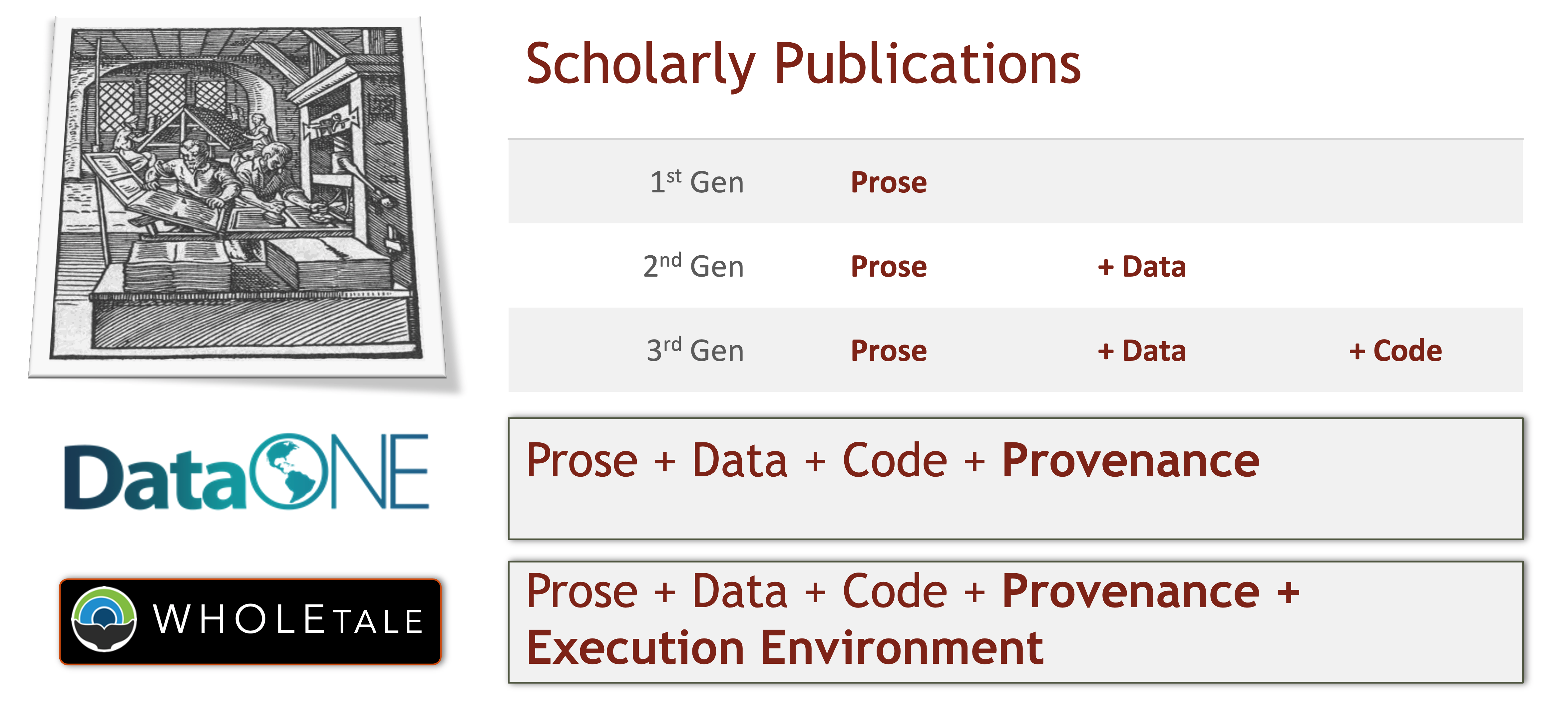
The 5th Generation
Whole Tale simplifies computational reproducibility. It enables researchers to easily package and share ‘tales’. Tales are executable research objects captured in a standards-based tale format complete with metadata. They can contain:
- data (references)
- code (computational methods)
- narrative (traditional science story)
- compute environment (e.g. RStudio, Jupyter)
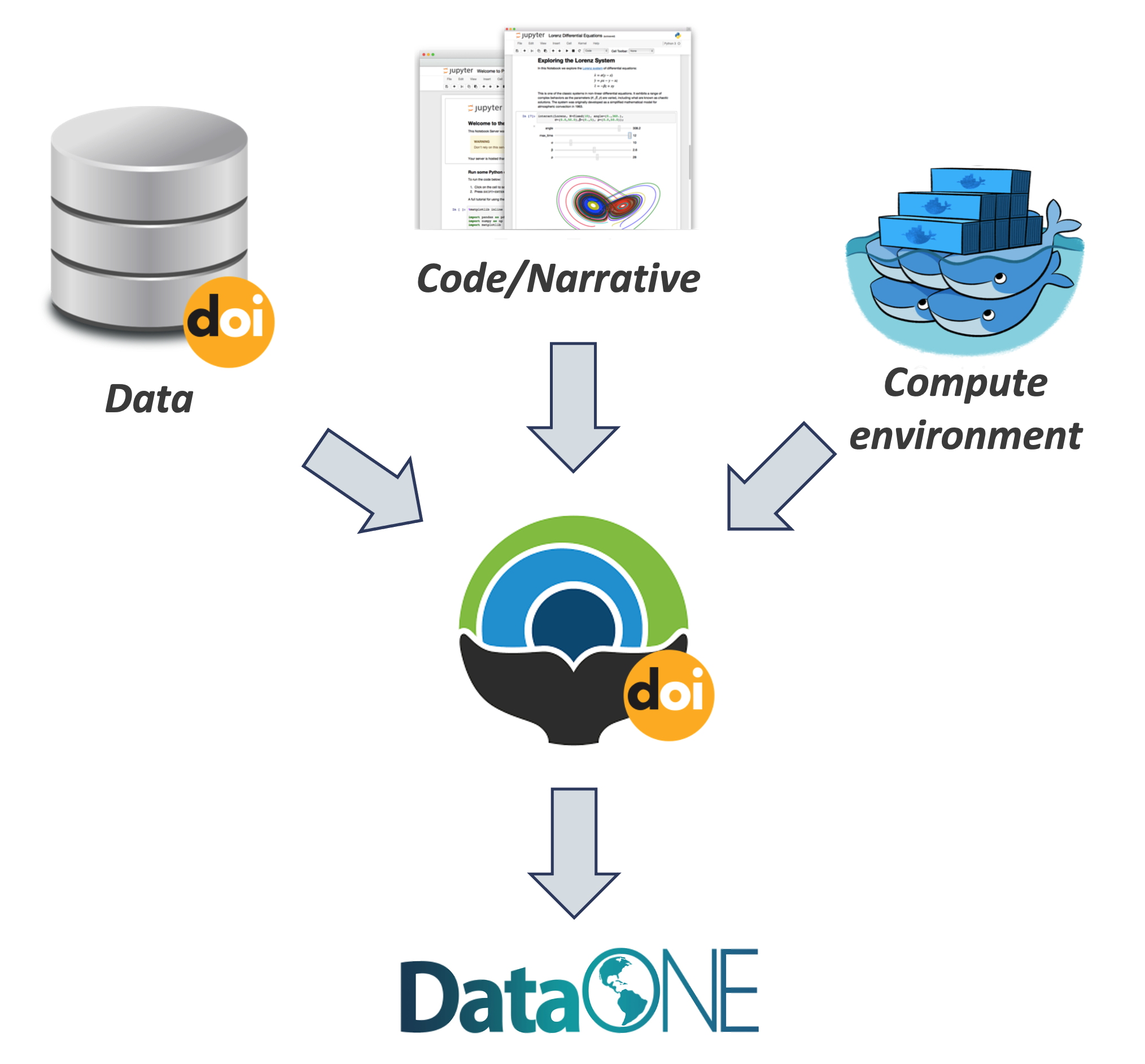
By combining data, code and the compute environment, tales allow researchers to:
- re-create the computational results from a scientific study
- achieve computational reproducibility
- “set the default to reproducible.”
They also empower users to verify and extend results with different data, methods, and environments. You can browse existing tales, run and interact with published tales and create new tales via the Whole Tale Dashboard.
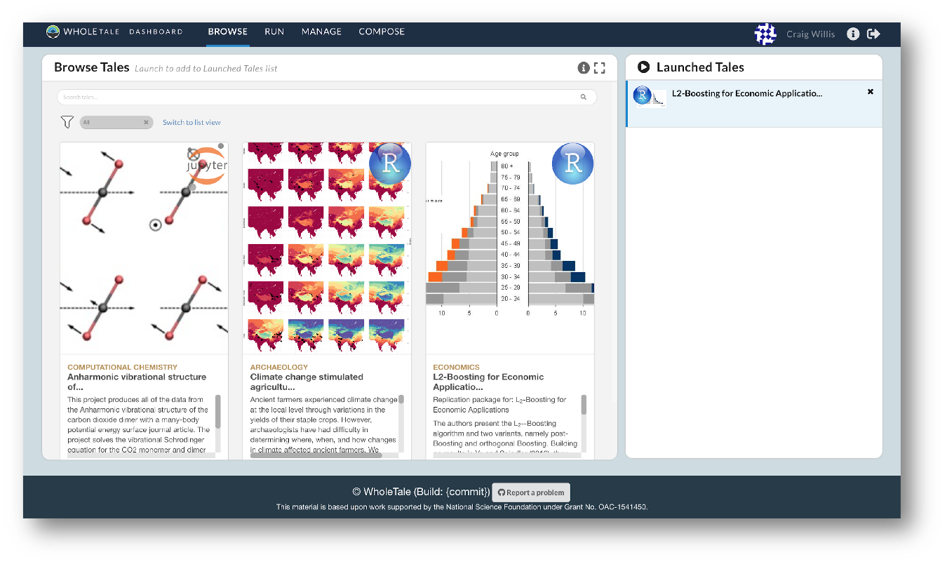
By integrating with DataONE and Dataverse, Whole Tale includes over 90 major research repositories from which a user can select datasets to make those datasets the starting point of an interactive data exploration and analysis inside of one of the Whole Tale environments. Within DataONE, we are adding functionality to work with data in the Whole Tale environment directly from the dataset landing page.
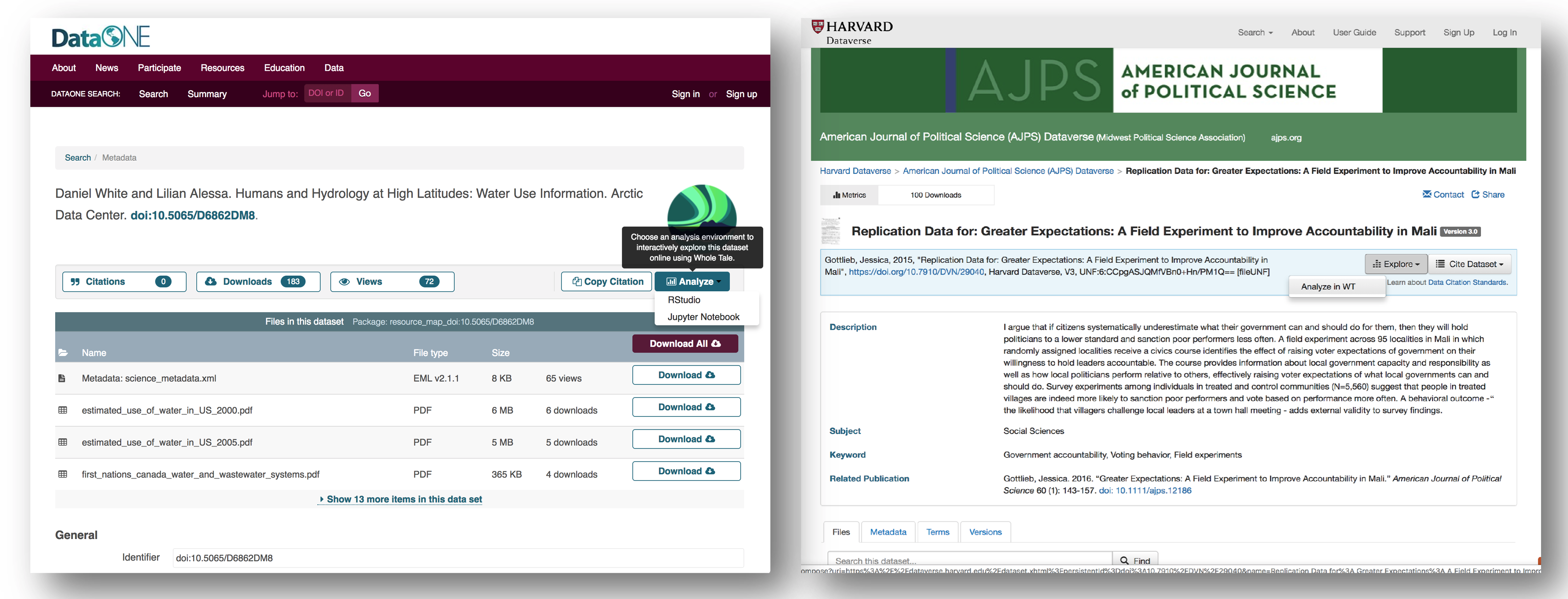
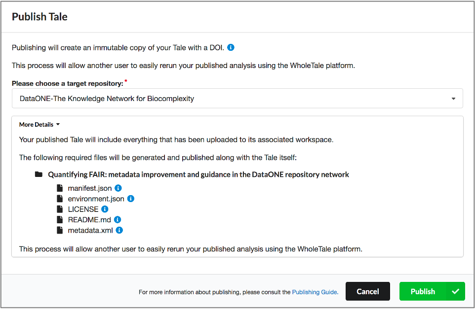 Full circle reproducibility can be achieved by publishing data, code AND the environment.
Borer, Elizabeth, Eric Seabloom, Matthew B. Jones, and Mark Schildhauer. 2009. “Some Simple Guidelines for Effective Data Management.” Bulletin of the Ecological Society of America 90: 205–14. https://doi.org/10.1890/0012-9623-90.2.205.
Hampton, Stephanie E, Sean Anderson, Sarah C Bagby, Corinna Gries, Xueying Han, Edmund Hart, Matthew B Jones, et al. 2015. “The Tao of Open Science for Ecology.” Ecosphere 6 (July). https://doi.org/http://dx.doi.org/10.1890/ES14-00402.1.
Munafò, Marcus R., Brian A. Nosek, Dorothy V. M. Bishop, Katherine S. Button, Christopher D. Chambers, Nathalie Percie du Sert, Uri Simonsohn, Eric-Jan Wagenmakers, Jennifer J. Ware, and John P. A. Ioannidis. 2017. “A Manifesto for Reproducible Science.” Nature Human Behaviour 1 (1): 0021. https://doi.org/10.1038/s41562-016-0021.
References
Borer, Elizabeth, Eric Seabloom, Matthew B. Jones, and Mark Schildhauer. 2009. “Some Simple Guidelines for Effective Data Management.” Bulletin of the Ecological Society of America 90: 205–14. https://doi.org/10.1890/0012-9623-90.2.205.
Hampton, Stephanie E, Sean Anderson, Sarah C Bagby, Corinna Gries, Xueying Han, Edmund Hart, Matthew B Jones, et al. 2015. “The Tao of Open Science for Ecology.” Ecosphere 6 (July). https://doi.org/http://dx.doi.org/10.1890/ES14-00402.1.
Munafò, Marcus R., Brian A. Nosek, Dorothy V. M. Bishop, Katherine S. Button, Christopher D. Chambers, Nathalie Percie du Sert, Uri Simonsohn, Eric-Jan Wagenmakers, Jennifer J. Ware, and John P. A. Ioannidis. 2017. “A Manifesto for Reproducible Science.” Nature Human Behaviour 1 (1): 0021. https://doi.org/10.1038/s41562-016-0021.