10 Session 10: Missing Data

10.1 Missing Data

10.1.1 General Concepts

a frequent problem
can bias estimates of parameters and their variances
lots of different ways to handle it
too often, solution is to throw out data - easiest, and easiest to justify.

But I am going review a few examples of how to get around missing data.

10.1.2 Where does missing data come from (or go?)

Types of missing data

10.1.3 What to do about missing data

How to record missing data

what does NULL mean? What does NA mean?
This is almost never specified. Some options:
- observation was not recorded, or was recorded and not entered
- data was collected and entered, but later found to be suspect, and removed
- the data is in my notebook / I can’t be bothered to enter it
- there was nothing to measure; a value here would not make sense

10.1.4 Types of missing data

The first two can be safely removed (Gelman and Hill 2006)

Missing completely at random. A useful assumption; difficult to prove.
Missing at random. Missingness depends on observed variables - e.g. one species of fish can be observed but not caught and measured, or a sensor only works when the temperature is below some threshold.
Missing not at random
Missing but depends on unobserved variable
Missing but depends on the variable itself

10.1.5 Approaches

If there are a few missing data points (<5-10%)

delete records with missing data
replace missing data If there are more, this can lead to bias.
MICE
Missing data in Bayesian models

10.1.5.1 MICE: Multiple Imputation by Chained Equations

This is one of the most commonly used approaches, because it is very powerful.

A few limitations of the MICE approach include: it requires the assumption that data are missing completely at random. Further, it is based on empirical analysis rather than theory.

Algorithm:

create multiple copies of data
impute missing values - use the distribution of a variable to impute plausible values for the missing data
perform analysis on the values
combine results

See Rubin 1987 and White et al 2011 for background on the MICE algorithm.

10.1.5.2 Interpolation

There are a variety of methods for interpolating missing data in time series. This is frequently used for environmental sensors - weather stations, eddy covariance towers, temperature or soil moisture data.

Lets look at an example. This dataset doesn’t have any missing data, so we will make some.

library(lubridate)
library(dplyr)
library(imputeTS)
library(forecast)
library(ggplot2)
theme_set(theme_bw())

mac_daymet <- readr::read_csv('../data/mac_daymet.csv') %>% 
    filter(year(date) > 2016)


mac_nas <- readr::read_csv('../data/mac_nas.csv')



ggplot(data = mac_daymet) + 
    geom_point(aes(date, tmean))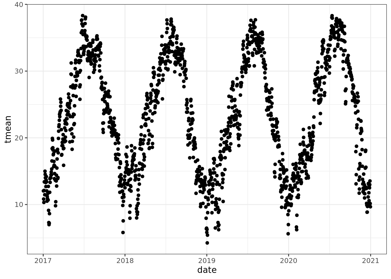

ggplot() + 
    geom_point(data = mac_daymet, aes(date, tmean), color = 'red', size = 1)+
    geom_point(data = mac_nas, aes(date, tmean), size = 1)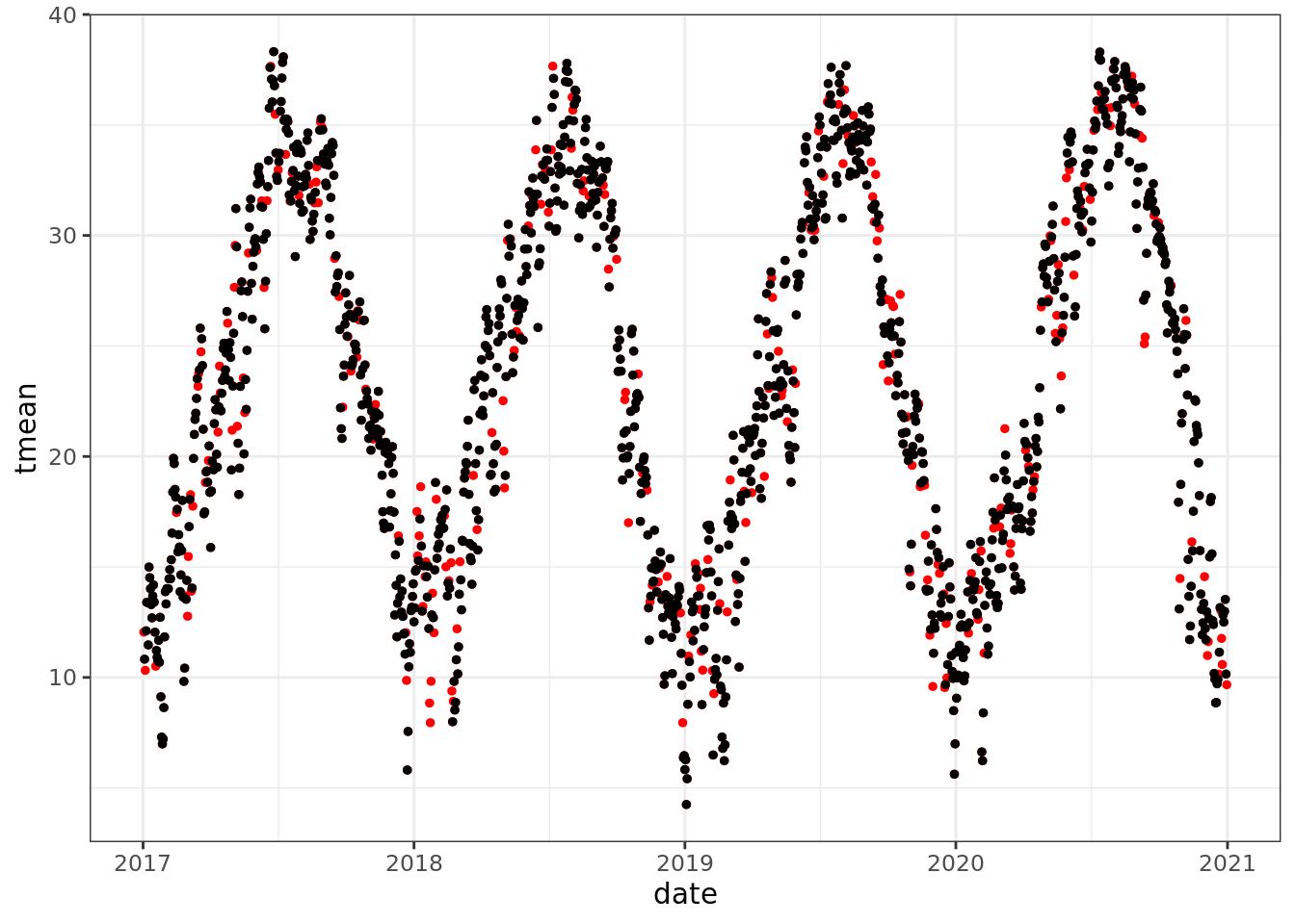

mac_nojja <- mac_daymet %>% 
    mutate(tmean = ifelse(month(date) %in% 6:8 & year(date) == 2020, NA, tmean))

ggplot() + 
    geom_point(data = mac_daymet, aes(date, tmean), color = 'red', size = 1)+
    geom_point(data = mac_nojja, aes(date, tmean), size = 1)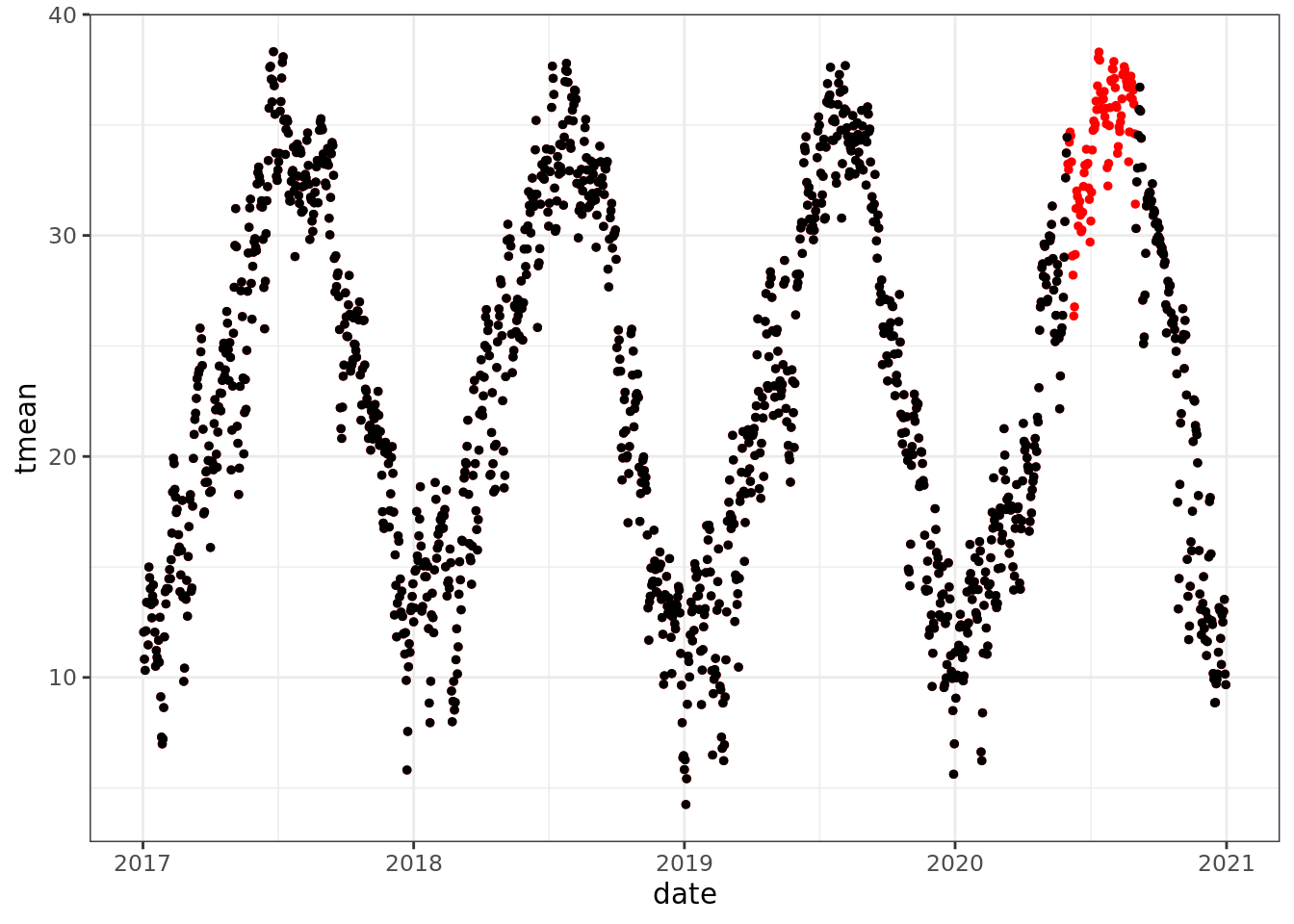

Now, what do we do?

Well, lets look for a related variable -

pairs(mac_daymet %>% filter(year(date) == 2020) %>% select(precip, tmin, tmean, vpd, date))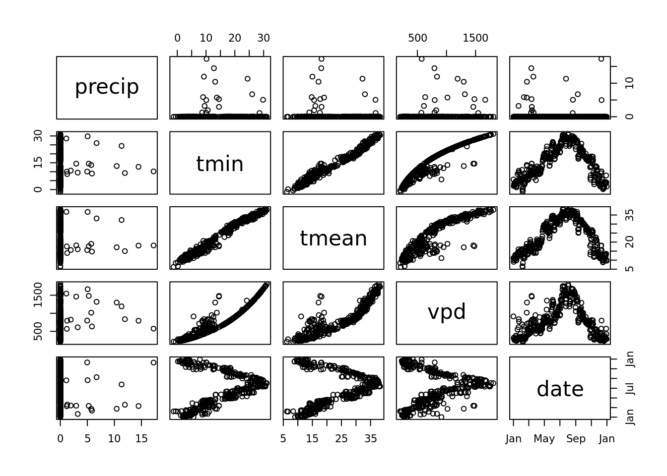

It looks like we can do a decent job of predicting tmean from tmin (or tmax for that matter … lets pretend that we don’t know the relationship tmean = (tmin + tmean) / 2 or have the ability to estimate )

tmean_model <- lm(tmean ~ tmin, data = mac_nas)

tmean_model2 <- lm(tmean ~ tmin + precip, data = mac_nas)

tmean_model3 <- lm(tmean ~ vpd + tmin, data = mac_nas)

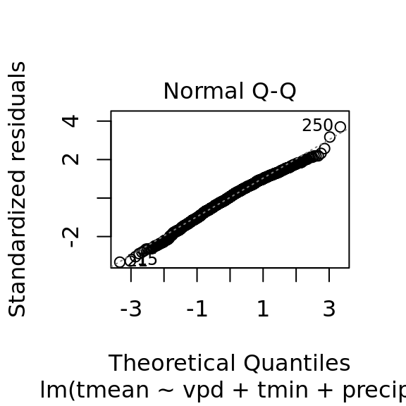
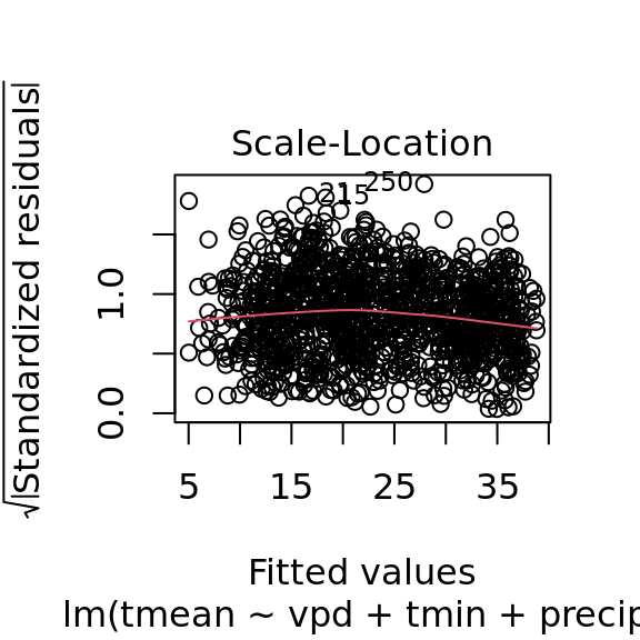
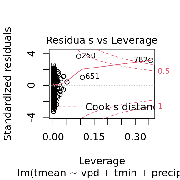
tmean_model4 <- lm(tmean ~ vpd + tmin + precip, data = mac_nas)

summary(tmean_model4)

## 
## Call:
## lm(formula = tmean ~ vpd + tmin + precip, data = mac_nas)
## 
## Residuals:
##     Min      1Q  Median      3Q     Max 
## -4.9949 -0.9598  0.0878  1.0588  5.2823 
## 
## Coefficients:
##               Estimate Std. Error t value Pr(>|t|)    
## (Intercept)  8.8403651  0.0996198  88.741  < 2e-16 ***
## vpd         -0.0018815  0.0001377 -13.663  < 2e-16 ***
## tmin         1.0703254  0.0077675 137.795  < 2e-16 ***
## precip      -0.1242346  0.0168094  -7.391 2.75e-13 ***
## ---
## Signif. codes:  0 '***' 0.001 '**' 0.01 '*' 0.05 '.' 0.1 ' ' 1
## 
## Residual standard error: 1.5 on 1184 degrees of freedom
##   (272 observations deleted due to missingness)
## Multiple R-squared:  0.9687, Adjusted R-squared:  0.9686 
## F-statistic: 1.221e+04 on 3 and 1184 DF,  p-value: < 2.2e-16

anova(tmean_model, tmean_model2, tmean_model3, tmean_model4)

## Analysis of Variance Table
## 
## Model 1: tmean ~ tmin
## Model 2: tmean ~ tmin + precip
## Model 3: tmean ~ vpd + tmin
## Model 4: tmean ~ vpd + tmin + precip
##   Res.Df    RSS Df Sum of Sq       F    Pr(>F)    
## 1   1186 3311.5                                   
## 2   1185 3086.1  1    225.48 100.150 < 2.2e-16 ***
## 3   1185 2788.7  0    297.34                      
## 4   1184 2665.7  1    122.98  54.624 2.751e-13 ***
## ---
## Signif. codes:  0 '***' 0.001 '**' 0.01 '*' 0.05 '.' 0.1 ' ' 1

### another way to check if we need the full model 
MASS::stepAIC(tmean_model4)

## Start:  AIC=968.15
## tmean ~ vpd + tmin + precip
## 
##          Df Sum of Sq   RSS    AIC
## <none>                 2666  968.1
## - precip  1       123  2789 1019.7
## - vpd     1       420  3086 1140.1
## - tmin    1     42750 45416 4334.6

## 
## Call:
## lm(formula = tmean ~ vpd + tmin + precip, data = mac_nas)
## 
## Coefficients:
## (Intercept)          vpd         tmin       precip  
##    8.840365    -0.001882     1.070325    -0.124235

### ok. both RSS and AIC say 'keep them all'!

nas <- which(is.na(mac_nas$tmean))

pred_tmean <- predict(object = tmean_model4, newdata = mac_nas[nas,])
mac_pred <- mac_nas
mac_pred$tmean[nas] <- pred_tmean

plot(tmean_model4)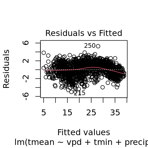

plot(pred_tmean, mac_daymet$tmean[nas]) +
  lines(0:40,0:40, lty = 2)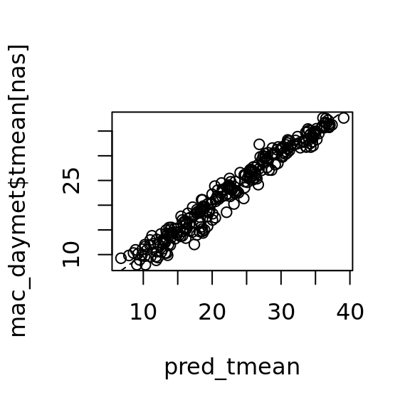

## integer(0)

hist(pred_tmean - mac_daymet$tmean[nas], breaks = 20)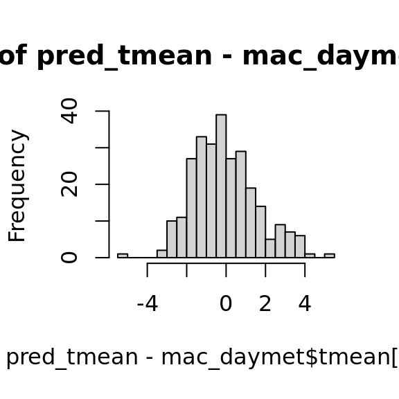

The book ’forecating practices and principles:

https://otexts.com/fpp2/missing-outliers.html

ggplot_na_imputations(x_with_na = mac_nojja$tmean, 
                      x_with_imputations = mac_pred$tmean, 
                      x_with_truth = mac_daymet$tmean )

ggplot_na_distribution(mac_nas$tmean, x_axis_labels = mac_nas$date)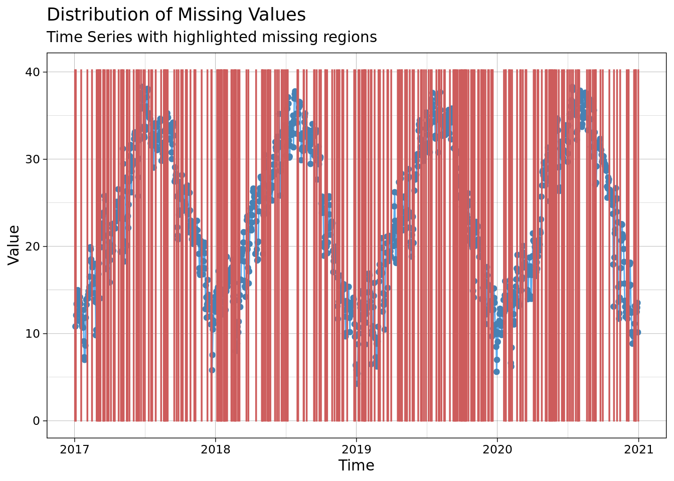

interp <- na.interp(mac_nas$tmean)

plot(mac_daymet$tmean, interp)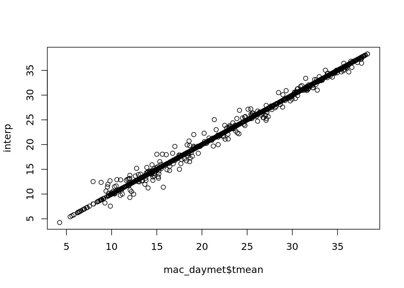

interp_jjas <- na.interp(mac_nojja$tmean)

plot(mac_daymet$tmean, interp_jjas)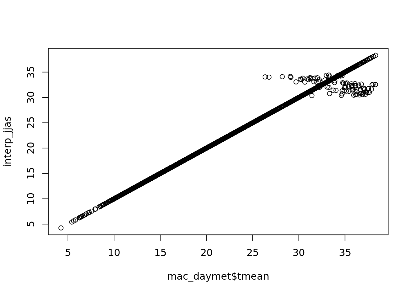

ggplot_na_distribution(mac_nas$tmean, x_axis_labels = mac_nas$date)

ggplot_na_distribution(mac_nojja$tmean, x_axis_labels = mac_nojja$date)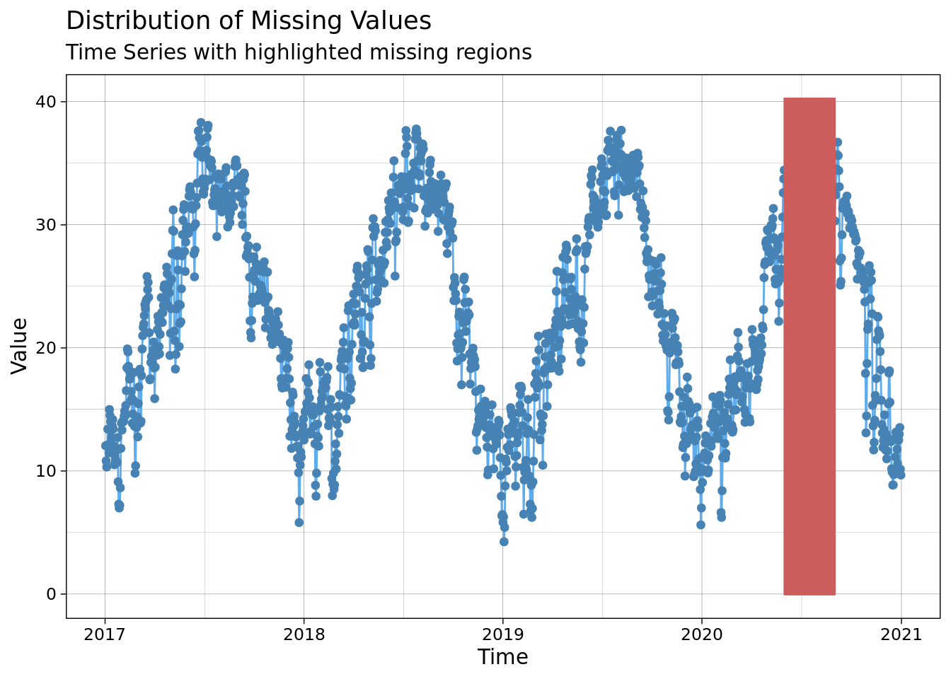

ggplot_na_intervals(mac_nas$tmean)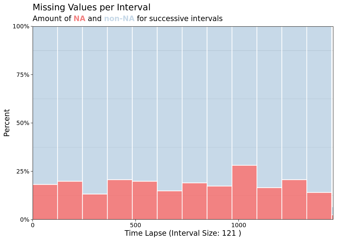

ggplot_na_intervals(mac_nojja$tmean)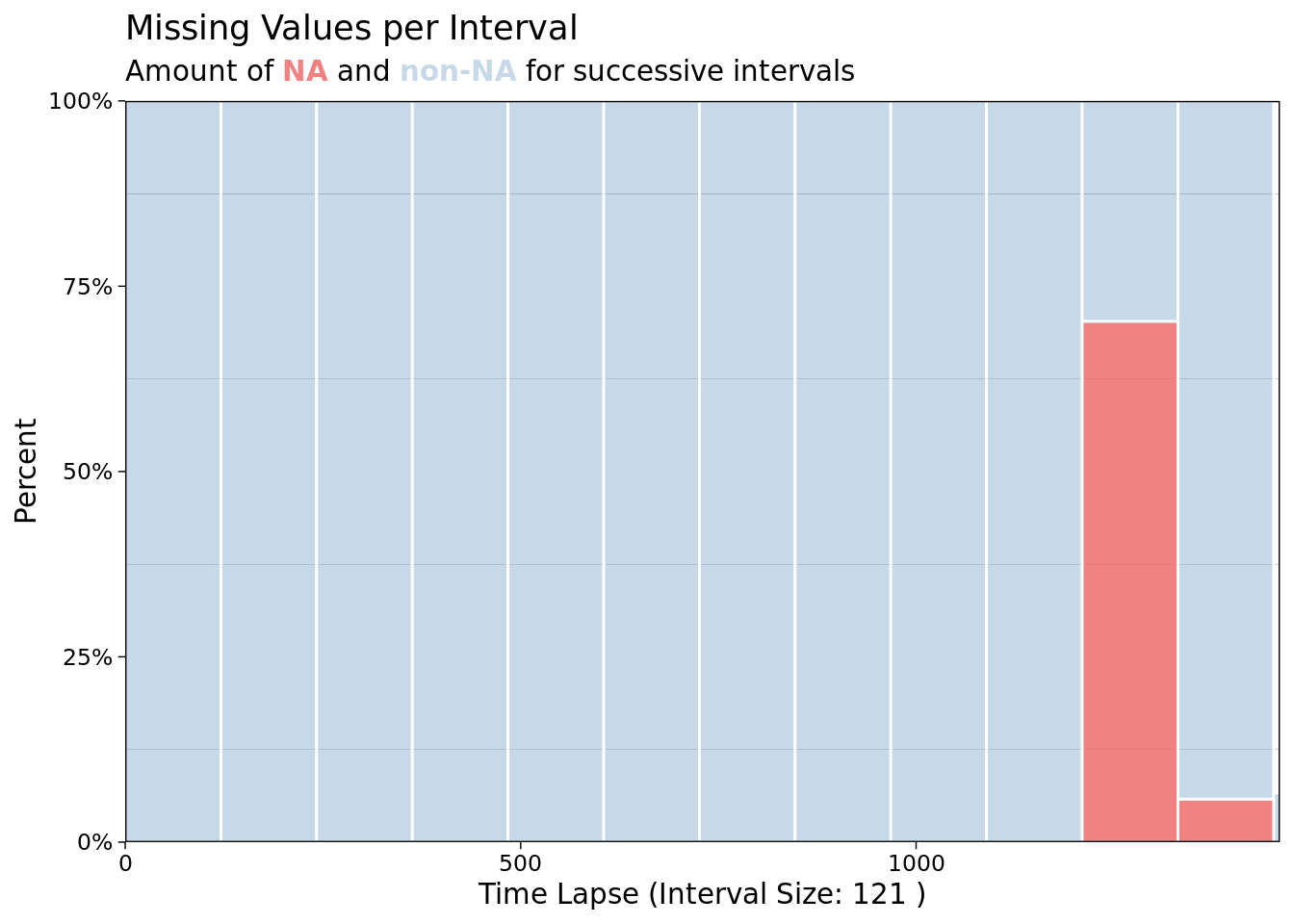

Gap Filling - weather, time series

imp <- na_interpolation(mac_nas, option = 'spline')
ggplot_na_imputations(x_with_na = mac_nas$tmean, x_with_imputations = imp$tmean, x_with_truth = mac_daymet$tmean )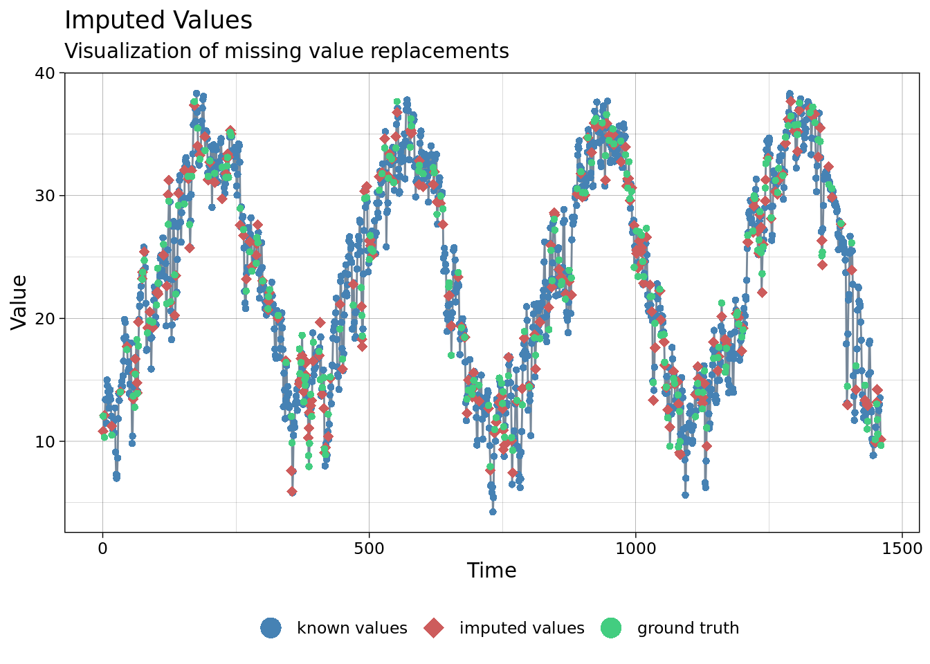

imp <- na_interpolation(mac_nojja, option = 'stine')
ggplot_na_imputations(x_with_na = mac_nojja$tmean, x_with_imputations = imp$tmean, x_with_truth = mac_daymet$tmean )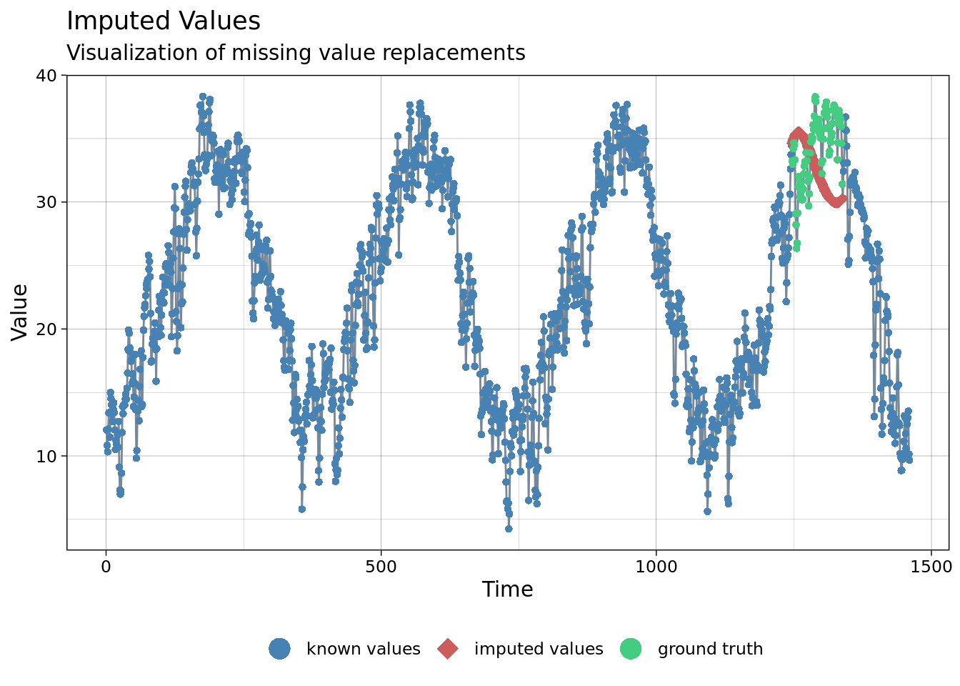

Your turn: try some different aproaches to missing data imputation:

replace with overall mean na_mean
replace with moving average na_ma
replace with … random draws? na_random

my_ts <- function(x){
    ts(x, start = c(2017, 1), 
       end = c(2020, 365), 
       deltat = 1/365)
}
    
imp <- na_seasplit(my_ts(mac_nojja$tmean))

ggplot_na_imputations(x_with_na = my_ts(mac_nojja$tmean), 
                      x_with_imputations = imp, 
                      x_with_truth = my_ts(mac_daymet$tmean ))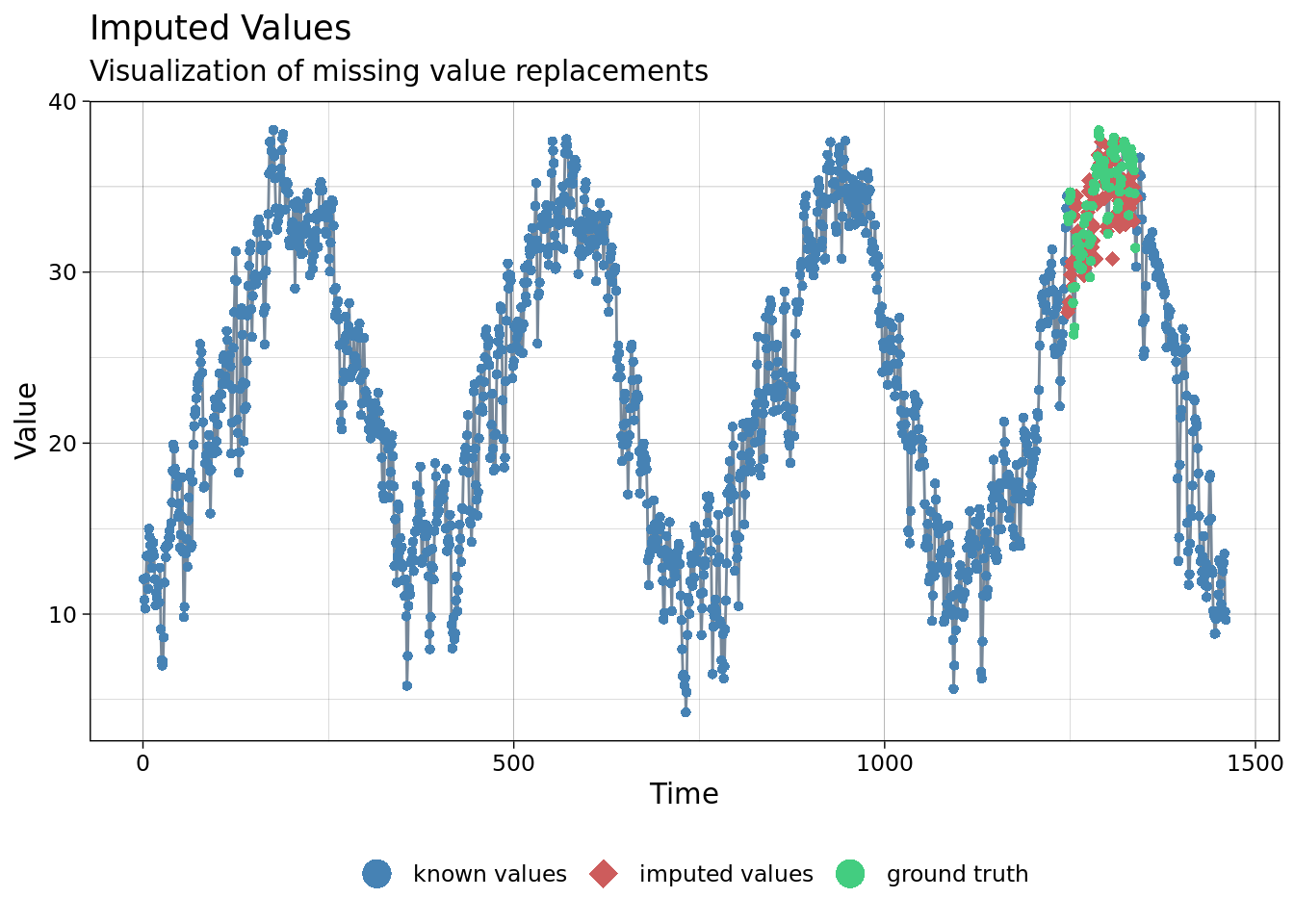

10.1.5.3 Bayesian Imputation

The brms package also provides utilities for handling missing data, including prior to model fitting using MICE and related methods as well as during model fitting. These are explained in the vignette by Brukner 2021 “Handle Missing Values with brms” and the online version of Statistical Rethinking Chapter 14.

The same can be done using JAGS, it is possible to estimate variables as model parameters during model fitting. With both JAGS and brms, it is necessary to specify a model for any variable with data being estimated (e.g. predictor variables must be explictly modeled as a response, even if drawn directly from a prior).

It is possible to use the MICE algorithm in Bayesian analysis. The disadvantage of using MICE with many Bayesian methods such as MCMC is that it increases the amount of computing time as a linear function of the number of datasets with imputed values (often 5-20x). Since many models can take hours or days to fit, this is an important limitation to consider.

10.1.5.4 Estimating SE from previously published findings to support Meta-analysis

A tangent: Meta-analysis itself can be viewed as a missing data problem. Combining information from two studies that were conducted in different conditions or treatment levels, I am trying to make inference about a single variable such as response rate even if the studies measured different responses. However, that is not the focus here.

Very often, meta-analysis models require measures of variance around a particular treatment response in order to weight the studies. However, the original studies have different goals than the meta-analysis, so these values may not be reported. A standard convention is to reject studies that do not have the required estimates of standard error. However, this can limit inference. It can also motivate sharing data - that would reduce the need for such laborious and uncertain approximations.

Some methods for estimating SE from other statistics are summarized in LeBauer 2020 (developed at the time of LeBauer et al 2013 but not given a doi until 2020), before the text Koricheva et al 2013 gave a related perspective. LeBauer et al 2013 also provide examples for estimating these statistics even where they can’t be estimated while fitting a meta-analysis.

10.1.6 References

Gelman and Hill 2006. Ch 25: Missing Data Imputation in “Data Analysis Using Regression and Multilevel/Hierarchical Models.” Cambridge University Press http://www.stat.columbia.edu/~gelman/arm/missing.pdf

Su, Y.-S., Gelman, A., Hill, J., & Yajima, M. (2011). Multiple Imputation with Diagnostics (mi) in R: Opening Windows into the Black Box. Journal of Statistical Software, 45(2), 1–31. https://doi.org/10.18637/jss.v045.i02 https://www.jstatsoft.org/article/view/v045i02

Rubin DB (1987). Multiple Imputation for Nonresponse in Surveys. John Wiley & Sons, New York.

White, Ian R., Patrick Royston, and Angela M. Wood. “Multiple imputation using chained equations: issues and guidance for practice.” Statistics in medicine 30.4 (2011): 377-399.

Steffen Moritz and Thomas Bartz-Beielstein (2017) imputeTS: Time Series Missing Value Imputation in R. The R Journal (2017) 9:1, pages 207-218. https://journal.r-project.org/archive/2017/RJ-2017-009/index.html

CRAN Task View: Missing Data https://cran.r-project.org/web/views/MissingData.html

Koricheva, J., Gurevitch, J., & Mengersen, K. (Eds.). (2013). Handbook of Meta-analysis in Ecology and Evolution. Princeton University Press. http://www.jstor.org/stable/j.ctt24hq6n

LeBauer, David S., et al. “Facilitating feedbacks between field measurements and ecosystem models.” Ecological Monographs 83.2 (2013): 133-154.

LeBauer, David. “Transforming ANOVA and Regression statistics for Meta-analysis.” Authorea Preprints (2020). https://doi.org/10.22541/au.158359749.96662550