An R package that allows users to create an interactive web application using R code. This packages calls for HTML, JavaScript and CSS without you having to learn them.
Think interactive web pages built by people who love to code in R, no JavaScript experience necessary.
“Shiny is an open source R package that provides an elegant and powerful web framework for building web applications using R. Shiny helps you turn your analyses into interactive web applications without requiring HTML, CSS, or JavaScript knowledge.” - Posit
The big benefits of Shiny is that you create an interactive web application just by understanding the Shiny framework in R and present all the cool visualization you create using R packages in an interactive platform.
Why build a Shiny App?
Rationale
Example
Share data in an engaging format, allowing your audience to interact with your data
HydroTech Helper by Daniel Kerstan. An app to access real-time monitoring of USGS hydrology sites.
To make tools you create in R accessible to others. Particularly those who do not know R. Instead of sharing your code, you share your app and everyone can see the output
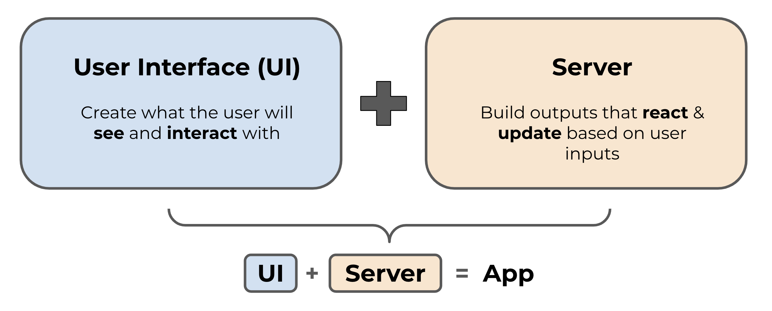
A web page that displays the app to a user (i.e. the user interface, or UI for short - frontend), and
A computer that powers the app (i.e. the server - backend)
Source: Intro to Shiny - Building reactive apps and dashboards, MEDS, UCSB
The UI controls the layout and appearance of your app and is written in HTML (but we use functions from the {shiny} package to write that HTML). The server handles the logic of the app – in other words, it is a set of instructions that tells the web page what to display when a user interacts with it.
Let’s take a look at how the code for a very simple Shiny app would look like to get a sense of the fundamental architecture of this tool.
library(shiny)# Define the UI1ui <- shiny::fluidPage("Hello there!")# Define the server2server <-function(input, output){ }# Generate the appshiny::shinyApp(ui = ui, server = server)
1
The fluidPage is a function that generates a page. It is important for allowing flexibility in UI layout which we’ll dive deeper later.
2
The server is actually a function with input and output as arguments. , where you’ll add all the code related to the computations.Because this app has no inputs or outputs, it doesn’t need anything in the ‘server’ component (though it still does require an “empty server”)
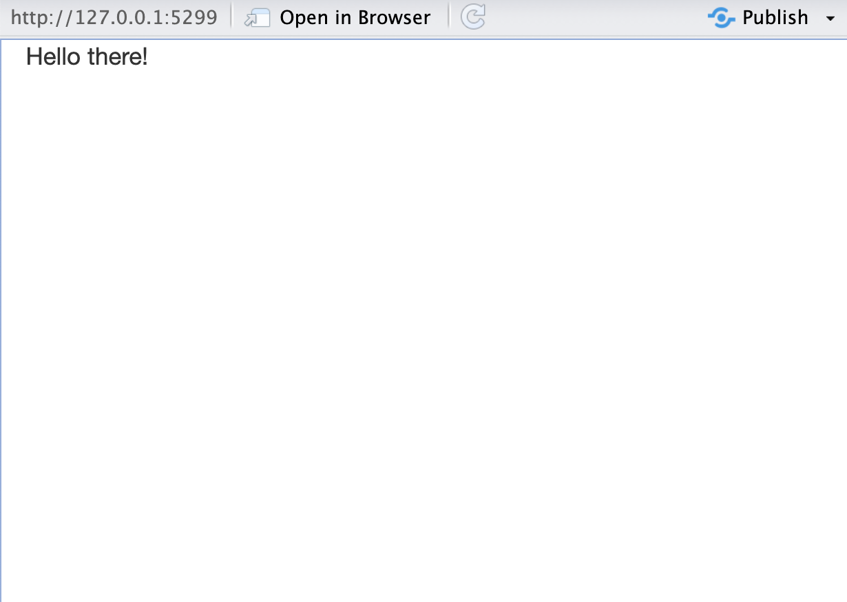
If we run the code above, we should see an app that is a blank white page with “Hello there!” written in the top left in plain text.
With this code we have essentially built a Shiny app. More complicated apps will certainly have more content in the UI and server sections but all Shiny apps will have this tripartite structure (Define UI, Define the Server and Generate the app).
15.2.2 What will go in each section?
Section
Component
UI
Inputs - or widgets ways the user can interact with (e.g. toggle, slide) and provide values to your app.
Outputs - The R objects that your user sees (e.g. tables, plots). Outputs respond when a user interacts with or changes an input value.
Layout - how the different components of the app are arranged.
Theme - defines the overall appearance of your app.
Server
Computations - code that will create the outputs displayed in your app (values, tables, plots, etc).
We are going to begin by focusing on understanding how the inputs and outputs work on the UI and how the sever operates to react based on inputs and display the outputs.
15.2.3 More on widgets and outputs
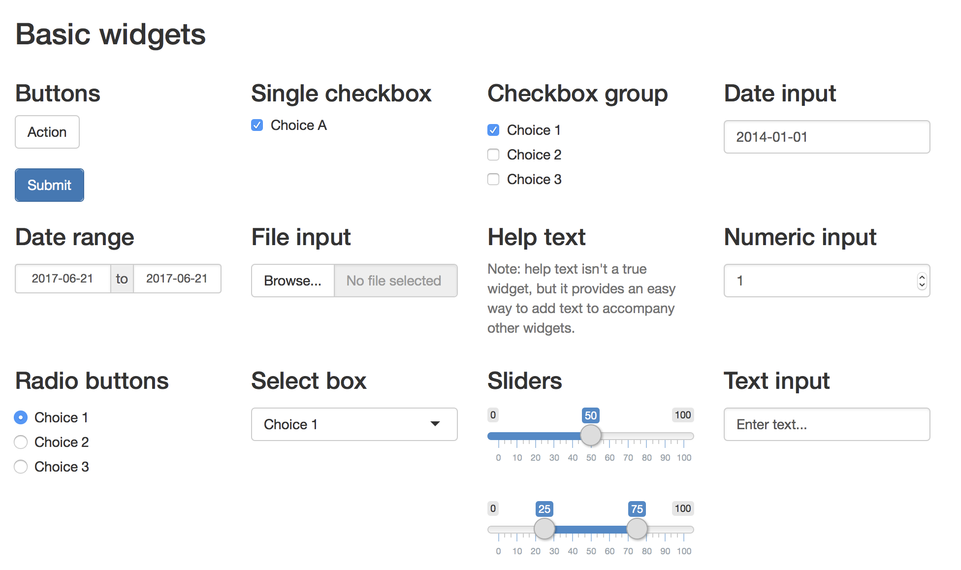
Widgets are web elements that users can interact with via the UI.
Widgets collect information from the user which is then used to update outputs created in the server. Shiny provides a set of standard widgets (see image below), but you can also explore widget extensions using a variety of other packages (e.g. {shinyWidgets}, {DT}, {plotly})
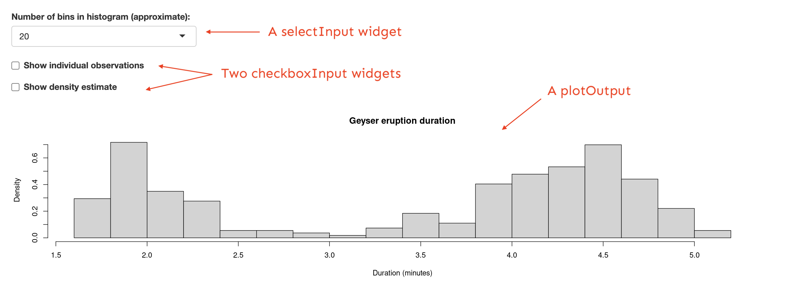
Outputs are R objects you will display on your app. This can be plots, tables, values, or others. Generally, these outputs are going to react to as the user interact with the inputs.
Example of input widgets and an output plot.
Source: Intro to Shiny - Building reactive apps and dashboards, MEDS, UCSB
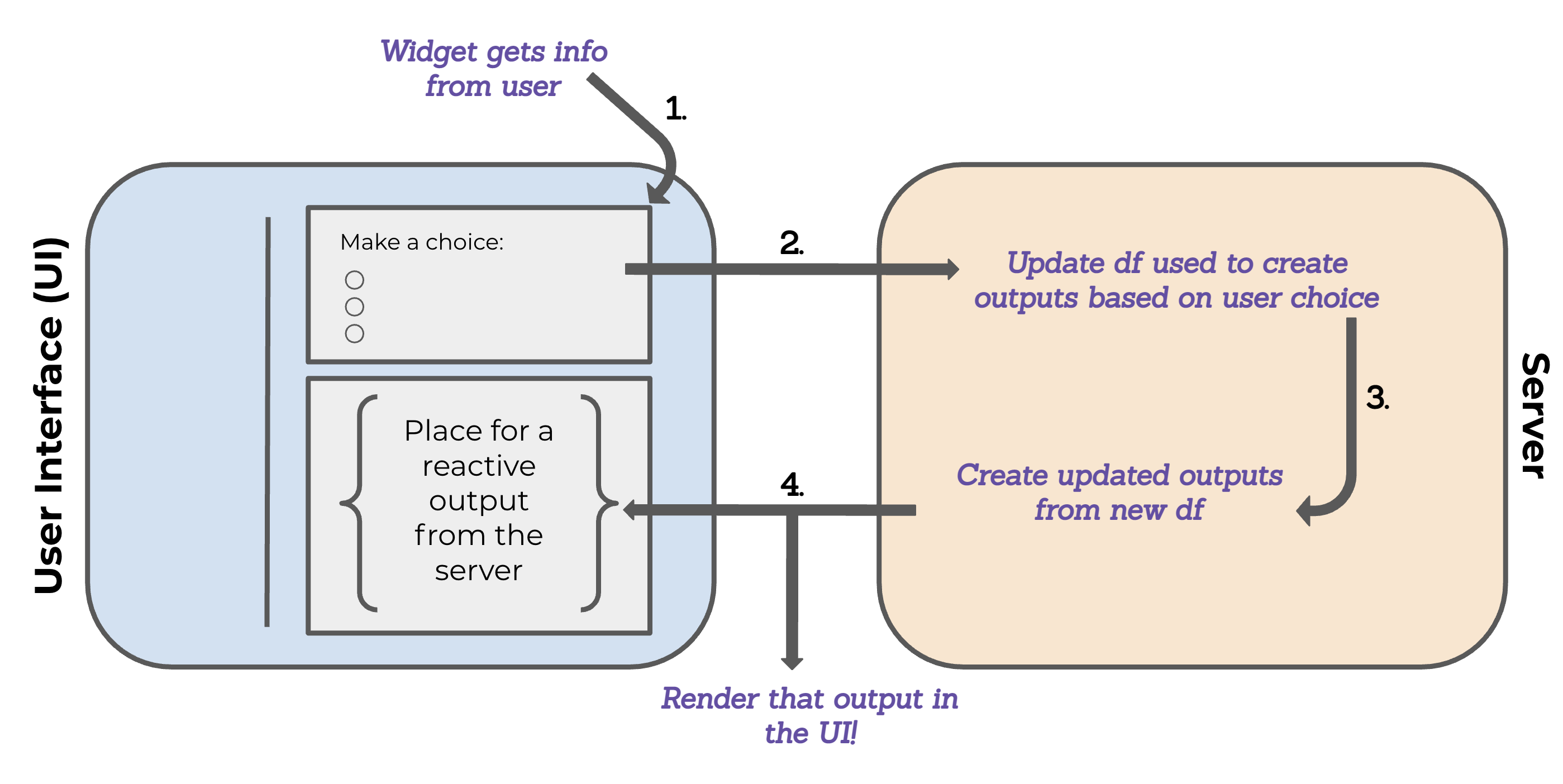
15.2.4 Reactivity: brief intro
Reactivity is what makes Shiny apps responsive i.e. it lets the app instantly update itself whenever the user makes a change. At a very basic level, it looks something like this:
Source: Intro to Shiny - Building reactive apps and dashboards, MEDS, UCSB
How to understand reactivity?
Check out Garrett Grolemund’s article, How to understand reactivity in R for a more detailed overview of Shiny reactivity.
15.3 How to organize our files when developing a Shiny app
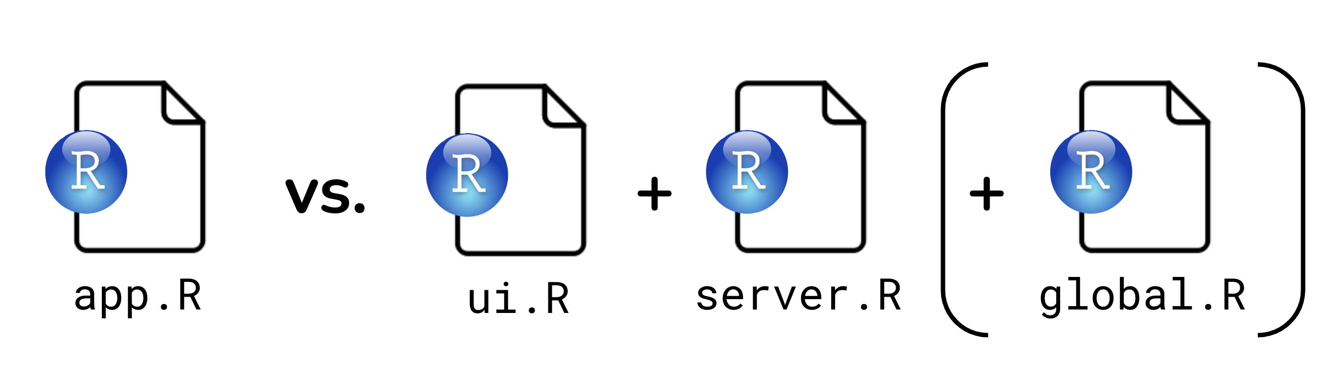
Before we jump into RStudio to create a Shiny app there a couple things worth mentioning about the structure of an app. First, when creating an app you have the option of either creating a single-file app or a two-file app. In both cases, the app looks the same, however the difference is you either have all the code for you app (ui + server) in one script named app.R or you have 2 files, one for ui (ui.R) and one for then server (server.R)
Source: Intro to Shiny - Building reactive apps and dashboards, MEDS, UCSB
Which one to choose?
It largely comes down to personal preference. A single-file format is best for smaller apps or when creating a reproducible example (reprex). While the two-file format is beneficial when writing large, complex apps where breaking apart code can make things a bit more navigable / maintainable.
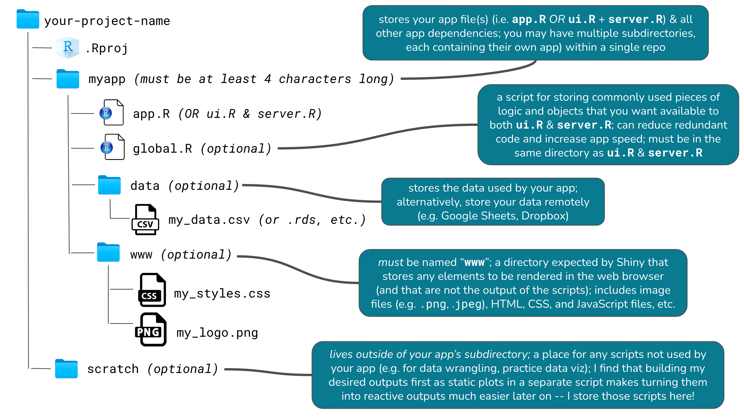
Second, as we have learned through this course, it is always a good idea to create a GitHub repository + an Rproj to house all the moving pieces of our app. The image below presents a general repo structure to stay organized. We will follow this structure for the apps we will create during this lesson.
Source: Intro to Shiny - Building reactive apps and dashboards, MEDS, UCSB
15.4 Creating a Shiny app
Set up: Create GitHub Repo
Create a repo to house our soon-to-be app(s). Navigate to your GitHub account, go to Your repositories > Click on New repository. Named it shiny-app-example Remember to initiate your repo with a README and choose R as the language for the default .gitignore.
Clone your repo into your RStudio Session in the server. Click on the green “< >Code” button > Copy the HTTPS url and then go to RStudio
In RStudio Create a new project. Go to File > New Project > Version Control with Git > paste Repository url > Create Project
The GIF bellow shows each of these steps as a visual reference. Thank you Sam Csik, who created this great resource!
You can create a single-file app using RStudio’s built-in Shiny app template (e.g. File > New Project > New Directory > Shiny Application), but it’s just as easy to create it from scratch (and you’ll memorize the structure faster!). Let’s do that now.
Set up: Your first Shiny app
In your project repo, create a sub-directory to house your app. Name it single-file-app. And a dub-directory for all our scratch code (e.g practice plots or subset df.)
Create a new R script inside single-file-app/ and name it app.R – you must name your script app.R.
Copy or type the following code into app.R, or use the shinyappsnippet to automatically generate a shiny app template.
# load packages ----library(shiny)# user interface ----ui <-fluidPage()# server instructions ----server <-function(input, output) {}# combine UI & server into an app ----shinyApp(ui = ui, server = server)
Tip: Use code sections (denoted by # some text ----) to make navigating different sections of your app code a bit easier. Code sections will appear in your document Outline (find the button at the top right corner of the script/editor panel).
Once you have saved your app.R file, the “Run” code button should turn into a “Run App” button. Click that button to run your app (alternatively, run runApp("directory-name") in your console.
runApp("single-file-app")
You won’t see much yet, as we have only built a blank app (but a functioning app, nonetheless!).
You should also notice a red stop sign appear in the top right corner of your console indicating that R is busy – this is because your R session is currently acting as your Shiny app server and listening for any user interaction with your app. Because of this, you won’t be able to run any commands in the console until you quit your app. To quit the app you have to press the stop button.
15.4.1 Building a single-file-app
We are now going to add elements to our base app. We will use data from {palmerpenguin} package and add the following features to our app:
A title and subtitle
A slider widget for users to select a range of penguin body masses
A reactive scatterplot that updates based on user-supplied values
Source: Intro to Shiny - Building reactive apps and dashboards, MEDS, UCSB
About {palmerpenguin}
The palmerpenguins data contains size measurements for three penguin species (Chinstrap, Gentoo and Adelie) observed on three islands in the Palmer Archipelago, Antarctica (Torgersen, Biscoe, and Dream).
15.4.2 Adding text to the UI: Title and Subtitle
We will do this in the UI withing fluidPage(). Remember this is a layout function that creates the basic visual structure of your app page.
Let’s add a title and subtitle to our app. Make sure they are separated with a coma!
# user interface ----ui <-fluidPage(# app title ----"My App Title",# app subtitle ----"Exploring Antarctic Penguin Data" )
15.4.3 Style text in the UI
The UI is actually an HTML document. We can style our text by adding static HTML elements using tags – a list of functions that parallel common HTML tags (e.g. <h1> == tags$h1()) The most common tags also have wrapper functions (e.g. h1()).
# user interface ----ui <-fluidPage(# app title ---- tags$h1("My App Title"), # alternatively, you can use the `h1()` wrapper function# app subtitle ----h4(strong("Exploring Antarctic Penguin Data")) # alternatively, `tags$h4(tags$strong("text"))` )
Adding intupts and outputs
Next, we will begin to add some inputs and outputs to our UI inside fluidPage(). Anything that you put into fluidPage() will appear in our app’s user interface. We want inputs and outputs to show up there.
Step 1: add an input to your app (slider widget)
# user interface ----ui <-fluidPage(# app title ---- tags$h1("My App Title"), # alternatively, you can use the `h1()` wrapper function# app subtitle ----h4(strong("Exploring Antarctic Penguin Data")), # alternatively, `tags$h4(tags$strong("text"))`# body mass slider input ----sliderInput(inputId ="body_mass_input", label ="Select a range of body masses (g):",min =2700, max =6300, value =c(3000, 4000)) )
Step 2: add an output “placeholder” in the UI
Outputs in the UI create placeholders which are later filled by the server function.
Similar to input functions, all output functions take the same first argument, outputId (note Id not ID), which connects the front end UI with the back end server. For example, if your UI contains an output function with an outputId = "plot", the server function will access it (or in other words, know to place the plot in that particular placeholder) using the syntax output$plot.
# user interface ----ui <-fluidPage(# app title ---- tags$h1("My App Title"), # alternatively, you can use the `h1()` wrapper function# app subtitle ----h4(strong("Exploring Antarctic Penguin Data")), # alternatively, `tags$h4(tags$strong("text"))`# body mass slider input ----sliderInput(inputId ="body_mass_input", label ="Select a range of body masses (g):",min =2700, max =6300, value =c(3000, 4000)),# body mass plot ouput ----plotOutput(outputId ="bodyMass_scatterplot_output") )
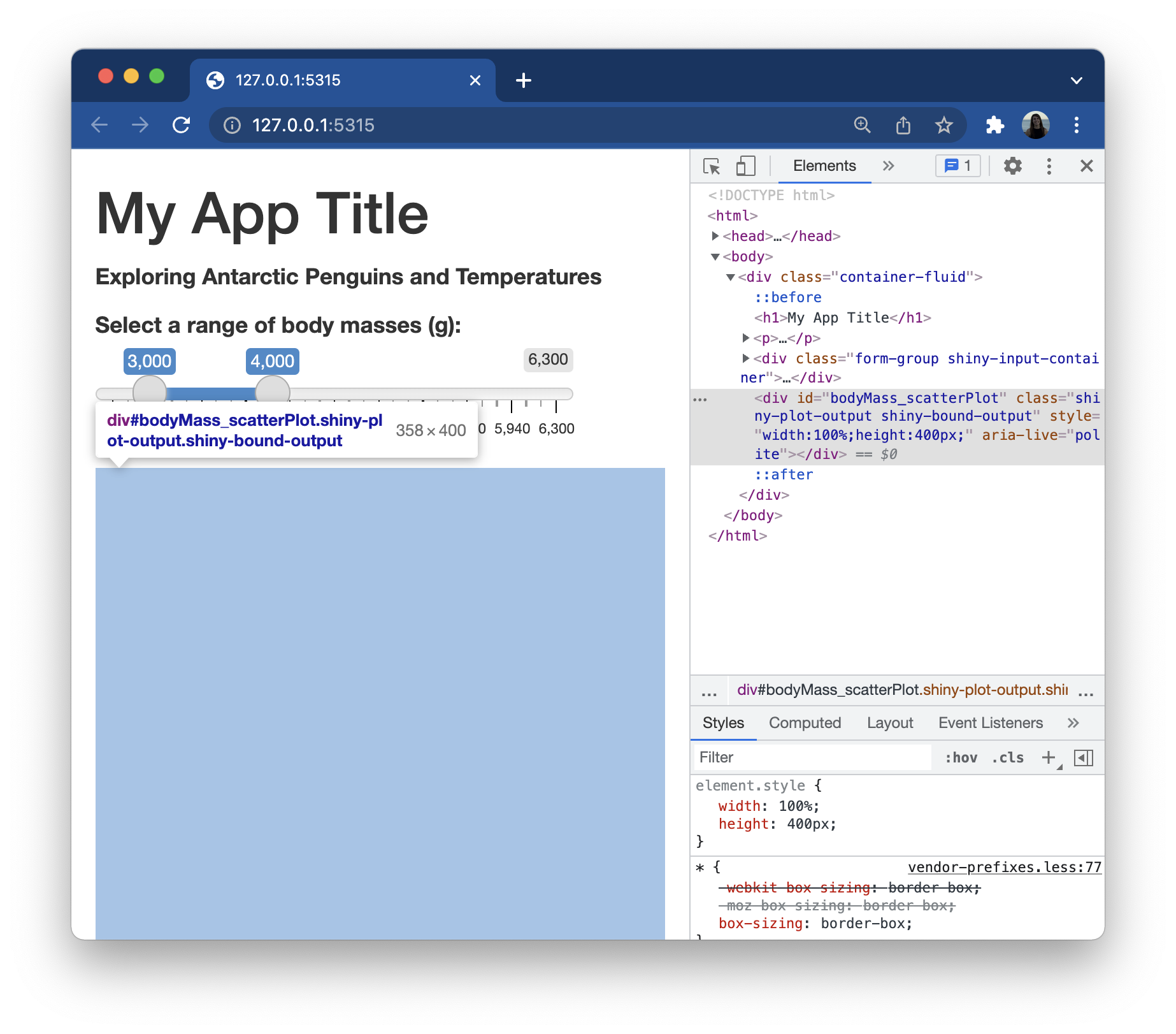
Okay, it looks like nothing changed?? Remember, *Output() functions create placeholders, but we have not yet written the server instructions on how to fill and update those placeholders. We can inspect the HTML and see that there is, in fact, a placeholder area awaiting our eventual output, which will be a plot named “bodyMass_scatterplot_output”:
Source: Intro to Shiny - Building reactive apps and dashboards, MEDS, UCSB
Tell the server how to assemble inputs into outputs: Adding reactive scatterplot
Now that we’ve designed our input / output in the UI, we need to write the server instructions (i.e. write the server function) on how to use the input value(s) (i.e. penguin body mass range via a slider input) to update the output (scatter plot).
The server function is defined with two arguments, input and output, both of which are list-like objects. You must define both of these arguments within the server function. input contains the values of all the different inputs at any given time, while output is where you’ll save output objects to be displayed in the app.
RULES
Save objects you want to display to output$<id>
Build reactive objects using a render*() function
Access input values with input$
Rule 1: Save objects you want to display to output$<id>
# load packages ----library(shiny)# user interface ----ui <-fluidPage(# ~ previous code omitted for brevity ~# body mass slider ----sliderInput(inputId ="body_mass_input", label ="Select a range of body masses (g):",min =2700, max =6300, value =c(3000, 4000)),# body mass plot output ----plotOutput(outputId ="bodyMass_scatterplot_output") )# server instructions ----server <-function(input, output) {# render penguin scatter plot ---- output$bodyMass_scatterplot_output <-# code to generate plot here}
Note: In the UI, our outputId is quoted (“bodyMass_scatterplot_output”), but not in the server (bodyMass_scatterplot_output).
Rule 2: Build reactive objects with render*()
Each *Output() function in the UI is coupled with a render*() function in the server, which contains the “instructions” for creating the output based on user inputs (or in other words, the instructions for making your output reactive).
Output function
Render function
dataTableOutput()
renderDataTable()
imageOutput()
renderImage()
plotOutput()
renderPlot()
tableOutput()
renderTable()
textOutput()
renderText()
# load packages ----library(shiny)# user interface ----ui <-fluidPage(# ~ previous code omitted for brevity ~# body mass slider ----sliderInput(inputId ="body_mass_input", label ="Select a range of body masses (g):",min =2700, max =6300, value =c(3000, 4000)),# body mass plot output ----plotOutput(outputId ="bodyMass_scatterplot_output") )# server instructions ----server <-function(input, output) {# render penguin scatter plot ---- output$bodyMass_scatterplot_output <-renderPlot({# code to generate plot here }) }
Aside: Write the code for the output objects in separate script first
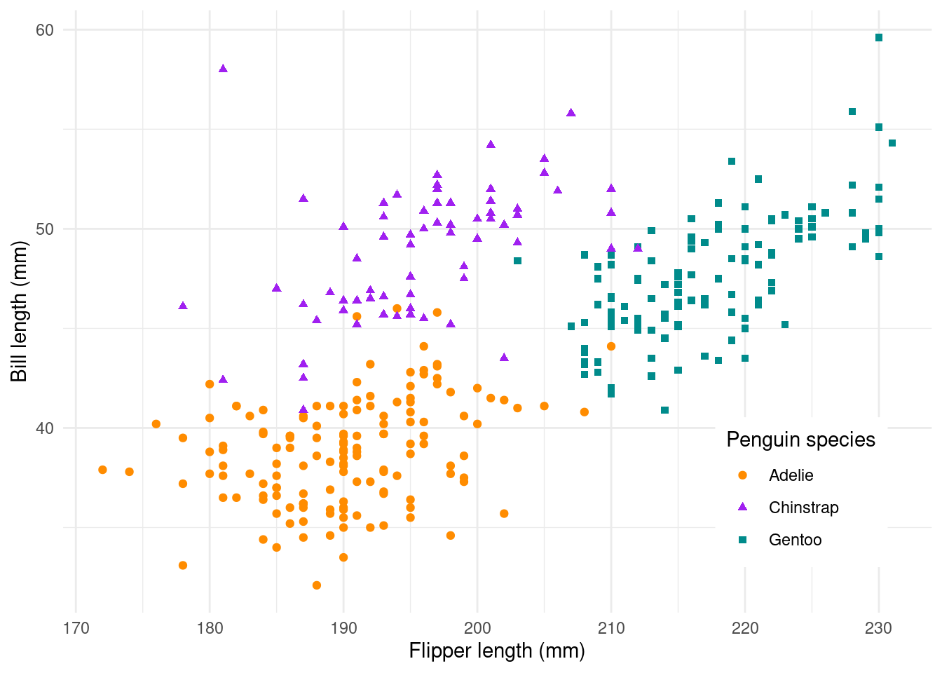
It is generally easier to experiment with the R objects you wan to show in your app (e.g. plots) in a separate script first and then copy the code over to your app. For example, if we want to make a scatter plot showing the relationship between flipper length and bill length for the different penguin species on palmerpenguins we would start by opening a new R script and write the code for this plot.
In RStudio, go to File > New File > RScript. Save this file as practice-script.R into the scratch folder. Now let’s copy and paste the code below. This code creates our scatter plot.
Copy your code over to your app, placing it inside the {} (and make sure to add any additional required packages to the top of your app.R script). Run your app. What do you notice?
# load packages ----library(shiny)library(palmerpenguins)library(tidyverse)# user interface ----ui <-fluidPage(# ~ previous code omitted for brevity ~# body mass slider ----sliderInput(inputId ="body_mass_input", label ="Select a range of body masses (g):",min =2700, max =6300, value =c(3000, 4000)),# body mass plot output ----plotOutput(outputId ="bodyMass_scatterplot_output"))# server instructions ----server <-function(input, output) {# render penguin scatter plot ---- output$bodyMass_scatterplot_output <-renderPlot({ ggplot(na.omit(penguins),aes(x = flipper_length_mm, y = bill_length_mm,color = species, shape = species)) +geom_point() +scale_color_manual(values =c("Adelie"="#FEA346", "Chinstrap"="#B251F1", "Gentoo"="#4BA4A4")) +scale_shape_manual(values =c("Adelie"=19, "Chinstrap"=17, "Gentoo"=15)) +labs(x ="Flipper length (mm)", y ="Bill length (mm)", color ="Penguin species", shape ="Penguin species") +theme_minimal() +theme(legend.position =c(0.85, 0.2), legend.background =element_rect(color ="white")) })}
Great! We have plot! But… It is not reactive. We have not yet told the server how to update the plot based on user inputs via the sliderInput() in the UI. Let’s do that next.
Aside: Practice filtering data in a separate script
Go back to out practice script practice-script.R and create a new data frame where we filter the body_mass_g column for observations within a specific range of values (in this example, values ranging from 3000 - 4000).
# filter penguins df for observations where body_mass_g >= 3000 & <= 4000 ----body_mass_df <- penguins %>%filter(body_mass_g %in%c(3000:4000))
Then, plot the new filtered data frame.
# plot new, filtered data ----ggplot(na.omit(body_mass_df), # plot 'body_mass_df' rather than 'penguins' dfaes(x = flipper_length_mm, y = bill_length_mm, color = species, shape = species)) +geom_point() +scale_color_manual(values =c("Adelie"="#FEA346", "Chinstrap"="#B251F1", "Gentoo"="#4BA4A4")) +scale_shape_manual(values =c("Adelie"=19, "Chinstrap"=17, "Gentoo"=15)) +labs(x ="Flipper length (mm)", y ="Bill length (mm)", color ="Penguin species", shape ="Penguin species") +theme_minimal() +theme(legend.position =c(0.85, 0.2),legend.background =element_rect(color ="white"))
Which part of our code needs to be updated when a user changes the slider range input?
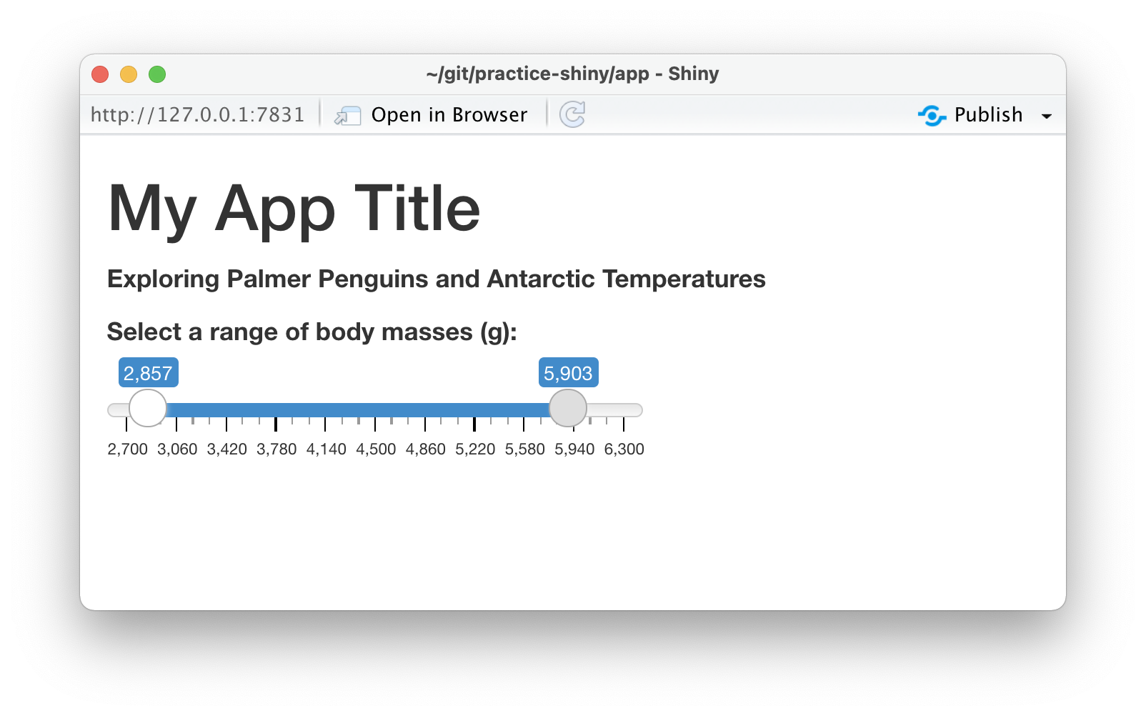
For example if someone inputs the following range:
Remember that in our UI we we gave the slidrInput() an inputID = body_mass_input.
# body mass slider ----sliderInput(inputId ="body_mass_input", label ="Select a range of body masses (g):", min =2700, max =6300, value =c(3000, 4000))
Now we need to add the input piece on the server side. We can access the values of that slider input in the server using the syntax, input$body_mass_input. If you want your output to change according to the input values, substitute hard-coded values (e.g. 2857:5903) with the input values from the UI. For example, c(input$body_mass_input[1]:input$body_mass_input[2]
Reactive Data Frame
We need to create a reactive data frame that is able to update according to the input. For this we use the reactive() function.
When you call your reactive data frame in your ggplot, the data frame name must be followed by ()
# load packages ----library(shiny)library(palmerpenguins)library(tidyverse)# user interface ----ui <-fluidPage(# ~ previous code omitted for brevity ~# body mass slider ----sliderInput(inputId ="body_mass_input", label ="Select a range of body masses (g):",min =2700, max =6300, value =c(3000, 4000)),# body mass plot output ----plotOutput(outputId ="bodyMass_scatterplot_output"))# server instructions ----server <-function(input, output) {# filter body masses ---- body_mass_df <-reactive({ penguins %>%filter(body_mass_g %in%c(input$body_mass_input[1]:input$body_mass_input[2])) })# render penguin scatter plot ---- output$bodyMass_scatterplot_output <-renderPlot({ ggplot(na.omit(body_mass_df()),aes(x = flipper_length_mm, y = bill_length_mm,color = species, shape = species)) +geom_point() +scale_color_manual(values =c("Adelie"="#FEA346", "Chinstrap"="#B251F1", "Gentoo"="#4BA4A4")) +scale_shape_manual(values =c("Adelie"=19, "Chinstrap"=17, "Gentoo"=15)) +labs(x ="Flipper length (mm)", y ="Bill length (mm)", color ="Penguin species", shape ="Penguin species") +theme_minimal() +theme(legend.position =c(0.85, 0.2), legend.background =element_rect(color ="white")) })}
Now let’s tun the app! We should now see a reactive Shiny app. Note that reactivity automatically occurs whenever you use an input value to render an output object.
15.4.4 Recap: Steps to create a reactive Shiny app
We created an app.R file in it’s own directory and began our app with the template, though you can also create a two-file Shiny app by using separate ui.R and server.R files.
We added an input to the fluidPage() in our UI using an *Input() function and gave it a unique inputId (e.g. inputId = "unique_input_Id_name")
We created a placeholder for our reactive object by using an *Output() function in the fluidPage() of our UI and gave it an outputId (e.g. outputId = "output_Id_name")
We wrote the server instructions for how to assemble inputs into outputs, following these rules:
Save objects that you want to display to output$<id>
Build reactive objects using a render*() function (and similarly, build reactive data frames using reactive() )
Access input values with input$<id>
And… we saw that reactivity automatically occurs whenever we use an input value to render an output object.
15.5 Your turn: Build on our 1-file app
Add another reactive widget
Working alone or in groups, add a reactive DT datatable to your app with a checkboxGroupInput (widget) that allows users to select which year(s) to include in the table. Configure your checkboxGroupInput so that the years 2007 and 2008 are pre-selected.
Remember that the DT package allows you to create interactive tables where you can filter, sort, and do lots of other neat things tables in HTML format.
Once you’ve added the new feature your app should look like this:
Source: Intro to Shiny - Building reactive apps and dashboards, MEDS, UCSB
Tips
Use ?checkboxGroupInput to learn more about which arguments you need (remember, all inputs require an inputId and oftentimes a label, but there are others required to make this work as well)
Both {shiny} and {DT} packages have functions named dataTableOutput() and renderDataTable() – The DT functions allows you to create both server-side and ui-side DataTables and supports additional DataTables features while Shiny functions only provides server-side DataTables. Be sure to use the ones from the {DT} package using the syntax packageName::functionName().
There are lots of ways to customize DT tables, but to create a basic one, all you need is DT::dataTable(your_dataframe)
Remember to follow the steps outlined above:
Add an input (e.g. checkboxGroupInput) to the UI that users can interact with.
Add an output (e.g. DT::datatableOutput) to the UI that creates a placeholder space to fill with our eventual reactive output.
Tell the server how to assemble inputs into outputs following 3 rules:
Save objects you want to display to output$<id>
Build reactive objects using a render*() function
Access input values with input$<id>
Exercise 1: A Solution
# load libraries ----library(shiny)library(tidyverse)library(DT)# user interface ----ui <-fluidPage(# app title ---- tags$h1("My App Title"), # alternatively, you can use the `h1()` wrapper function# app subtitle ----h4(strong("Exploring Antarctic Penguin Data")), # alternatively, `tags$h4(tags$strong("text"))`# body mass slider input ----sliderInput(inputId ="body_mass_input", label ="Select a range of body masses (g):",min =2700, max =6300, value =c(3000, 4000)),# body mass plot output ----plotOutput(outputId ="bodyMass_scatterplot_output"),# year checkbox input ----checkboxGroupInput(inputId ="year_select", label ="Select year(s)" ,choices =c(2007, 2008, 2009),selected =c(2007, 2008)),# interactive table output ---- DT::dataTableOutput(outputId ="interactive_table_output"))# server instructions ----server <-function(input, output) {# filter body masses ---- body_mass_df <-reactive({ penguins %>%filter(body_mass_g %in%c(input$body_mass_input[1]:input$body_mass_input[2])) })# reactive scatterplot --- output$bodyMass_scatterplot_output <-renderPlot({ggplot(na.omit(body_mass_df()),aes(x = flipper_length_mm, y = bill_length_mm,color = species, shape = species)) +geom_point() +scale_color_manual(values =c("Adelie"="#FEA346", "Chinstrap"="#B251F1", "Gentoo"="#4BA4A4")) +scale_shape_manual(values =c("Adelie"=19, "Chinstrap"=17, "Gentoo"=15)) +labs(x ="Flipper length (mm)", y ="Bill length (mm)", color ="Penguin species", shape ="Penguin species") +theme_minimal() +theme(legend.position =c(0.85, 0.2), legend.background =element_rect(color ="white")) })# reactive-table ---- penguins_years <-reactive({ penguins %>%filter(year %in%c(input$year_select)) }) output$interactive_table_output <- DT::renderDataTable( DT::datatable(penguins_years(),options =list(pagelength =10),rownames =FALSE) )}# combine UI & server into an app ----shinyApp(ui = ui, server = server)
Common Mistakes
We all make mistakes! Specially when building a Shiny app. Here a few common mistakes to be on the lookout:
Misspelling inputId as inputID (or outputId as outputID)
Misspelling your inputId (or outputId) name in the server (e.g. UI: inputId = "myInputID", server: input$my_Input_ID)
Repeating inputIds (each must be unique)
Forgetting to separate UI elements with a comma, ,. Commas are a thing in Shiny.
Forgetting the set of parentheses when calling the name of a reactive data frame (e.g. ggplot(my_reactive_df, aes(...)) should be ggplot(my_reactive_df(), aes(...)) )
15.6 Layouts
So far, we have created an app that is perfectly functional, but it’s not so visually pleasing. Nothing really grabs your eye, inputs & outputs are stacked vertically on top of one another (which requires a lot of vertical scrolling), widget label text is difficult to distinguish from other text.
Source: Intro to Shiny - Building reactive apps and dashboards, MEDS, UCSB
To improve the looks of out app we used Layout functions. Layout functions provide the high-level visual structure of your app. Layouts are created using a hierarchy of function calls (typically) inside fluidPage(). Layouts often require a series functions – container functions establish the larger area within which other layout elements are placed. Let’s look at a few examples:
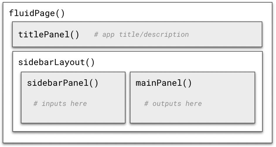
To create a page with a side bar and main area that contain your inputs and outputs (respectively). This format allows for really clear visual separation between where you want the user to interact with the app versus where the results of their choices can be viewed. Explore the following layout functions and read up on the sidebarLayout documentation.
fluidPage(titlePanel(# app title/description ),sidebarLayout(sidebarPanel(# inputs here ),mainPanel(# outputs here ) ))
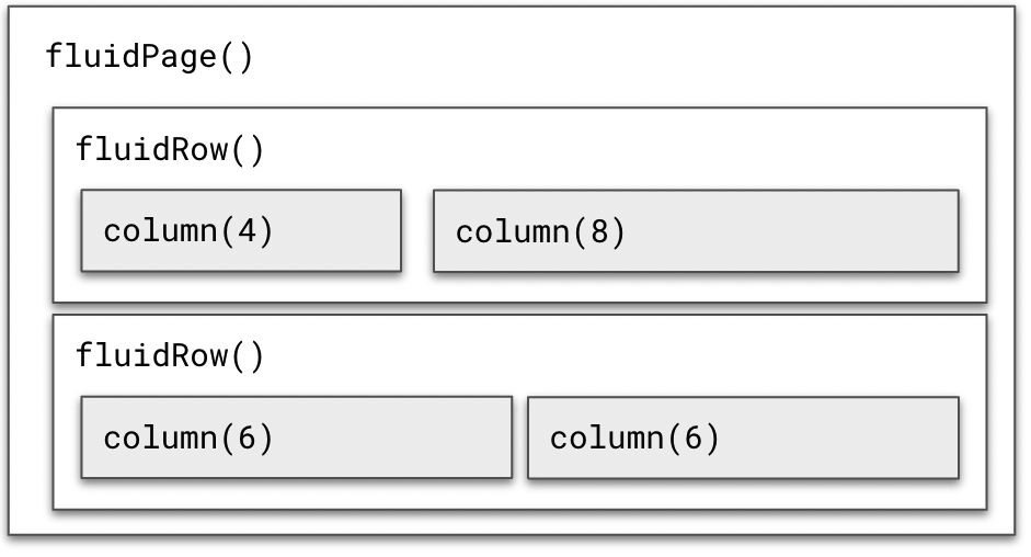
To create a page with multiple rows, explore the following layout functions and check out the fluid layout documentation. Note that each row is made up of 12 columns. The first argument of the column() function takes a value of 1-12 to specify the number of columns to occupy.
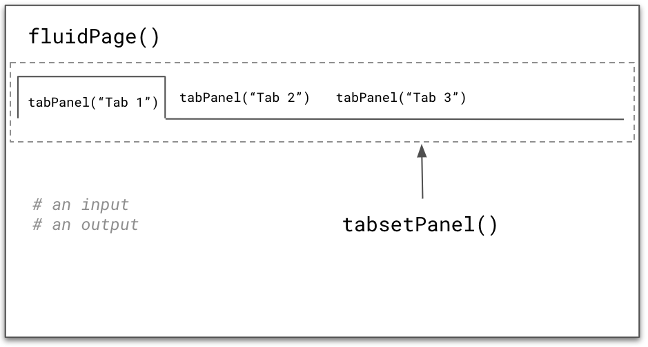
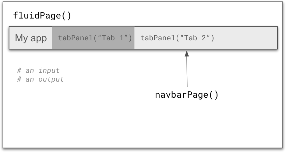
You may find that you eventually end up with too much content to fit on a single application page. Enter tabsetPanel() and tabPanel(). tabsetPanel() creates a container for any number of tabPanel()s. Each tabPanel() can contain any number of HTML components (e.g. inputs and outputs). Find the tabsetPanel documentation here and check out this example.
tabsetPanel(tabPanel("Tab 1", # an input# an output ),tabPanel("Tab 2"),tabPanel("Tab 3"))
You may also want to use a navigation bar (navbarPage()) with different pages (created using tabPanel()) to organize your application. Read through the navbarPage documentation and try running the example below.
navbarPage(title ="My app",tabPanel(title ="Tab 1",# an input# an output ),tabPanel(title ="Tab 2"))
More on Layouts
Experimenting with different app layouts can be a fun step in the process of making an app that is as effective as possible! It is important to remark that layouts are exclusively an element of the UI! This is great when you have an app with a complicated server component because you won’t need to mess with that at all to get the UI looking perfect.
Let’s create a “nicer” looking app by adding some layouts and additional formatting. We will start from scratch and build an app using a ui.R file and a server.R file. Additionally, we will create a global.R to demonstrate how what can go into this file.
The idea for this app is to look something like this:
Setup
We will start by creating a new folder in our shiny-app-example project. In the project’s directory create a new folder and name it two-file-app.
Inside the two-file-app folder create the three main files: ui.R, sever.R and global.R
Tips for success
Enable rainbow parentheses: Tools > Global Options > Code > Display > check Use rainbow parentheses
Add code comments at the start and end of each UI element: Even with rainbow parentheses, it can be easy to lose track or mistake what parentheses belong with which (see examples on follow slide)
Add placeholder text within your layout functions: Adding text, like “slider input will live here” and “plot output here” will help you better visualize what you’re working towards. It also makes it easier to navigate large UIs as you begin adding real inputs and outputs.
Use keyboard shortcuts to realign your code: Select all your code using cmd / ctrl + A, then realign using cmd / ctrl + I.
Build a Navar with two pages
ui <-navbarPage(title ="Palmer Penguins Data Explorer",# (Page 1) intro tabPanel ----tabPanel(title ="About this App","background info will go here"# REPLACE THIS WITH CONTENT ), # END (Page 1) intro tabPanel# (Page 2) data viz tabPanel ----tabPanel(title ="Explore the Data","inputs and outputs will live here"# REPLACE THIS WITH CONTENT ) # END (Page 2) data viz tabPanel) # END navbarPage
Tip: Run your app often while building out your UI to make sure it’s looking as you’d expect!
Add a fluidPage and 2 sidebarLayout to “Explore the Data” page
In one sidebarLayout we will add a plot and in the other a table.
# (Page 2) data viz sidebalLayout ----tabPanel(title ="Explore the Data",fluidPage(# penguin plot sidebarLayout ----sidebarLayout("Penguin plot goes here" ), # END penguin plot sidebarLayout# penguin table sidebarLayout ----sidebarLayout("Penguin tables goes here" ) # END penguin table sidebarLayout ) # END Fuild Page ) # END (Page 2) data viz tabPanel)# END navbarPage
Add sidebar & main panels in sidebarLayouts
We’ll eventually place our input in the sidebar and output in the main panel.
# (Page 2) data viz sidebalLayout ----tabPanel(title ="Explore the Data",fluidPage(# penguin plot sidebarLayout ----sidebarLayout(sidebarPanel("Plot input goes here"#REPLACE WITH CONTENT ),mainPanel("Penguin plot output goes here"#REPLACE WITH CONTENT ), ), # END penguin plot sidebarLayout# penguin table sidebarLayout ----sidebarLayout(sidebarPanel("Table input goes here"#REPLACE WITH CONTENT ),mainPanel("Penguin table output goes here"#REPLACE WITH CONTENT ) ) # END penguin table sidebarLayout ) # END Fuild Page ) # END (Page 2) data viz tabPanel)# END navbarPage
Add packages to global.R
We are introducing 2 new packages this time. {shinyWidgets} which provided us with more widget options, and {markdown} which will help us format text in a much more straight forward way.
# LOAD LIBRARIES ----library(shiny)library(palmerpenguins)library(tidyverse)library(shinyWidgets)library(markdown)library(leaflet)## Here you could also read in your data! Any data frame created in the global.R will be available to accesss in the server.
Add plot inputs
First, a shinyWidgets::pickerInput() that allows users to filter data based on island, and that includes buttons to Select All / Deselect All island options at once.
# penguin plot sidebarLayout ----sidebarLayout(# penguin plot sidebarPanel ----sidebarPanel(# island pickerInput ----pickerInput(inputId ="penguin_island_input", label ="Select an island(s):",choices =c("Torgersen", "Dream", "Biscoe"),selected =c("Torgersen", "Dream", "Biscoe"),options =pickerOptions(actionsBox =TRUE),multiple =TRUE), # END island pickerInput
Add shiny::sliderInput() that allows users to change the number of histogram bins and that by default, displays a histogram with 25 bins
# penguin plot sidebarLayout ----sidebarLayout(# penguin plot sidebarPanel ----sidebarPanel(# island pickerInput ----pickerInput(inputId ="penguin_island_input", label ="Select an island(s):",choices =c("Torgersen", "Dream", "Biscoe"),selected =c("Torgersen", "Dream", "Biscoe"),options =pickerOptions(actionsBox =TRUE),multiple =TRUE), # END island pickerInput# bin number sliderInput ----sliderInput(inputId ="bin_num_input", label ="Select number of bins:",value =25, max =100, min =1), # END bin number sliderInput ), # END penguin plot sidebarPanel
Add a plot output to the UI
Next, we need to create a placeholder in our UI for our trout scatterplot to live. Because we’ll be creating a reactive plot, we can use the plotOutput() function to do so.
# penguin plot mainPanel ----mainPanel(plotOutput(outputId ="flipperLength_histogram_output") ) # END penguin plot mainPanel), # END penguin plot sidebarLayout
Tell the server how to assemble pickerInput & sliderInput values into your plotOutput
Remember the three rules for building reactive outputs:
save objects you want to display to output$<id>
build reactive objects using a render*() function
access input values with input$<id>
(This is also when we will go to our scratch script to practice the necessary wrangling or creating the necessary plot. For this time, we are going to copy the code from the book )
# filter for island ----island_df <-reactive({ penguins %>%filter(island %in% input$penguin_island_input)})# render the flipper length histogram ----output$flipperLength_histogram_output <-renderPlot({ggplot(na.omit(island_df()), aes(x = flipper_length_mm, fill = species)) +geom_histogram(alpha =0.6, position ="identity", bins = input$bin_num_input) +scale_fill_manual(values =c("Adelie"="#FEA346", "Chinstrap"="#B251F1", "Gentoo"="#4BA4A4")) +labs(x ="Flipper length (mm)", y ="Frequency",fill ="Penguin species") +theme_light() +theme(axis.text =element_text(color ="black", size =12),axis.title =element_text(size =14, face ="bold"),legend.title =element_text(size =14, face ="bold"),legend.text =element_text(size =13),legend.position ="bottom",panel.border =element_rect(colour ="black", fill =NA, linewidth =0.7))})
Run the app and try out your widgets!
Your Turn
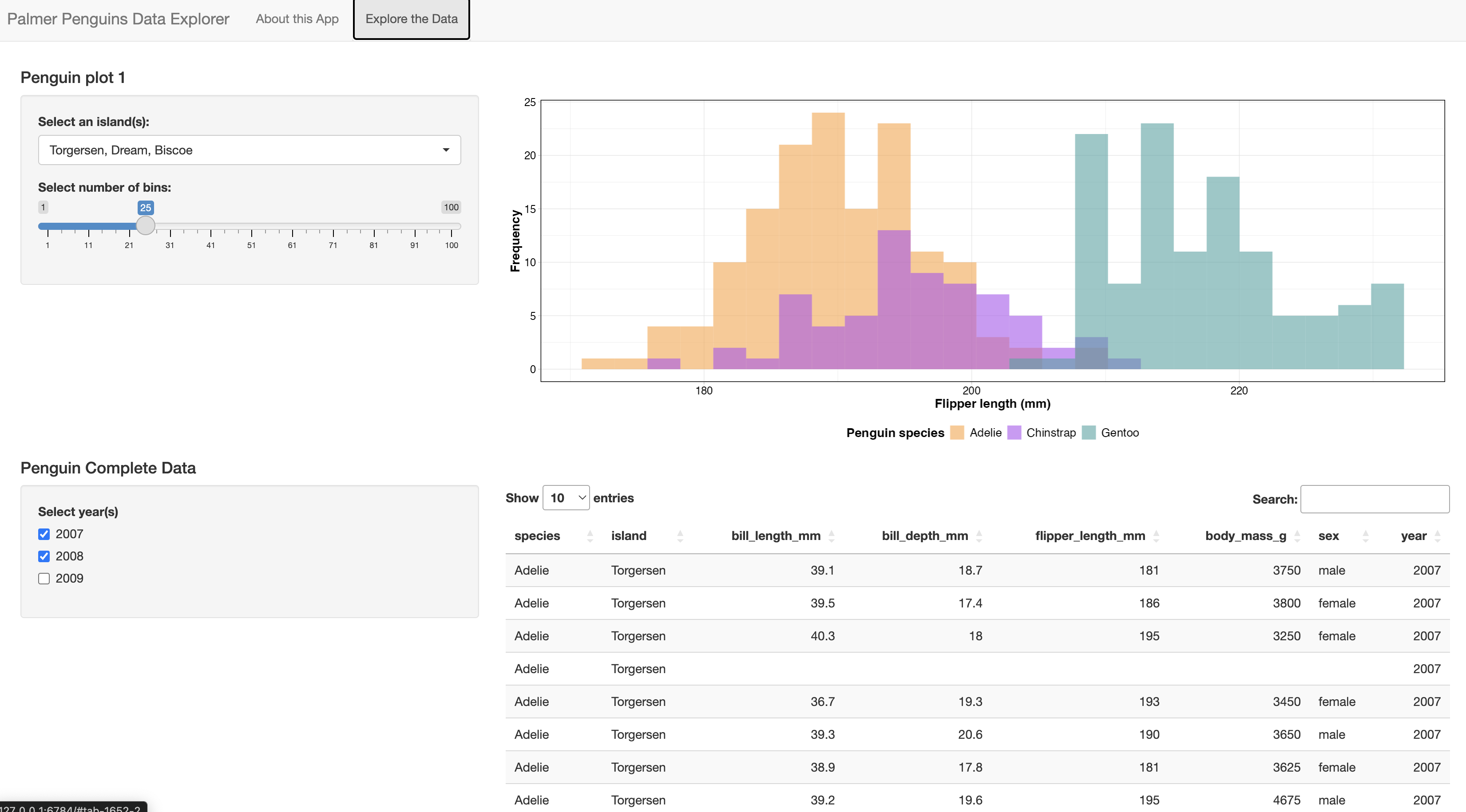
Add input and output to create an interactive table in the Explore Data panel
Working alone or in groups, add a reactive DT datatable to your app with a checkboxGroupInput (widget) that allows users to select which year(s) to include in the table. Configure your checkboxGroupInput so that the years 2007 and 2008 are pre-selected.
Remember that the DT package allows you to create interactive tables where you can filter, sort, and do lots of other neat things tables in HTML format.
Once you’ve added the new feature your app should look like this:
High-level steps
Create the checkboxGroupInput inside the sidebarPanel()
Add plot output to the UI in the mainPanel(). Use DT::dataTableOutput()
Tell the server how to render the table (FOLLOW THE 3 RULES, hint: DT::renderDataTable() is the function that pairs with dataTableOutput().
Exercise 2 Solution: UI
# penguin table sidebarLayout ----sidebarLayout(# penguin table sidebarPanel ----sidebarPanel(# year checkbox input ----checkboxGroupInput(inputId ="year_select", label ="Select year(s)" ,choices =c(2007, 2008, 2009),selected =c(2007, 2008)), # END checkbox input ), # END penguin table sidebarPanel# penguin table mainPanel ----mainPanel( DT::dataTableOutput(outputId ="interactive_table_output") ) # END penguin table mainPanel) # END penguin table sidebarLayout
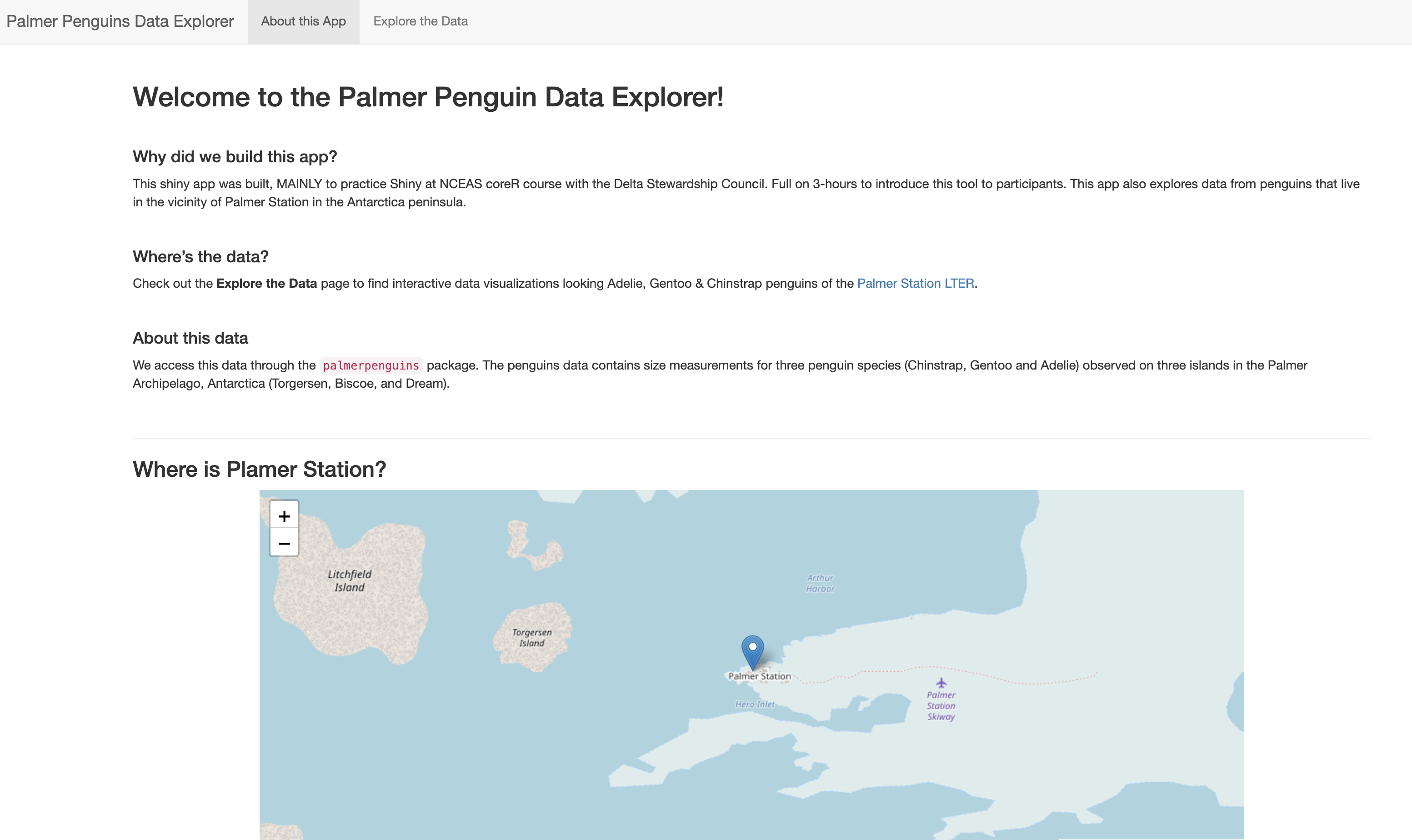
Let’s finalize this app: Adding information in About page
It is generally a good idea to add some context, background or other relevant information to your app. In this case we are going to add a description of the app and the data used, plus a Leaflet map showing Palmer Station.
Adding long text to the UI can get very confusing given that we need to use HTML wrapper functions for everything we write. This is when the {markdown} packages comes in handy. This package allows at to call an.md` file with text written and formatted in Markdown. Let’s see how it works.
We will start by creating a folder call text inside our app folder. Then we will create an .md file and save it into the text folder. To create an .md file go to: File > New File > Text file. Then save this file in the text folder and name it about.md.
Inside this file we are going to paste the following text
## Welcome to the Palmer Penguin Data Explorer!

<br>

#### Why did we build this app?

This shiny app was built, MAINLY to practice Shiny at NCEAS coreR course with the Delta Stewardship Council. Full on 3-hours to introduce this tool to participants. This app also explores data from penguins that live in the vicinity of Palmer Station in the Antarctica peninsula.


<br>

#### Where's the data?

Check out the **Explore the Data** page to find interactive data visualizations looking Adelie, Gentoo & Chinstrap penguins of the [Palmer Station LTER](https://pallter.marine.rutgers.edu/).

<br>

#### About this data
We access this data through the [`palmerpenguins`](https://allisonhorst.github.io/palmerpenguins/) package. The penguins data contains size measurements for three penguin species (Chinstrap, Gentoo and Adelie) observed on three islands in the Palmer Archipelago, Antarctica (Torgersen, Biscoe, and Dream).

<br>
<hr>


### Where is Plamer Station?
Next, we need to call this file from the UI.
# (Page 1) intro tabPanel ----tabPanel(title ="About this App",# intro text fluidRow ----fluidRow(# use columns to create white space on sidescolumn(1),column(10, includeMarkdown("text/about.md")),column(1) ), # END intro text fluidRow
Finally, we will add a Leaflet map in the About pane to indicate where Palmer Station is located.
Step 1 is to create the place holder in the UI by creating a leafletOutput.
fluidRow(## create column with leaflet outputcolumn(2),column(8, leafletOutput(outputId ="palmer_station_map")),column(2) )
Step 2, is to add the instructions on the server following the 3 rules.
save objects you want to display to output$<id>
build reactive objects using a render*() function
access input values with input$<id>
In this case we don’t need to call any input, given that the map is not reacting to any user’s input.
ui <-navbarPage(title ="Palmer Penguins Data Explorer",# (Page 1) intro tabPanel ----tabPanel(title ="About this App",# intro text fluidRow ----fluidRow(# use columns to create white space on sidescolumn(1),column(10, includeMarkdown("text/about.md")),column(1) ), # END intro text fluidRowfluidRow(## create column with leaflet outputcolumn(2),column(8, leafletOutput(outputId ="palmer_station_map")),column(2) ) ), # END (Page 1) intro tabPanel# (Page 2) data viz sidebalLayout ----tabPanel(title ="Explore the Data",fluidPage(h4("Penguin plot 1"),# penguin plot sidebarLayout ----sidebarLayout(# penguin plot sidebarPanel ----sidebarPanel(# island pickerInput ----pickerInput(inputId ="penguin_island_input", label ="Select an island(s):",choices =c("Torgersen", "Dream", "Biscoe"),selected =c("Torgersen", "Dream", "Biscoe"),options =pickerOptions(actionsBox =TRUE),multiple =TRUE), # END island pickerInput# bin number sliderInput ----sliderInput(inputId ="bin_num_input", label ="Select number of bins:",value =25, max =100, min =1), # END bin number sliderInput ), # END penguin plot sidebarPanel# penguin plot mainPanel ----mainPanel(plotOutput(outputId ="flipperLength_histogram_output") ) # END penguin plot mainPanel ), # END penguin plot sidebarLayout# Penguin table title ----h4("Penguin Complete Data"),# penguin table sidebarLayout ----sidebarLayout(# penguin table sidebarPanel ----sidebarPanel(# year checkbox input ----checkboxGroupInput(inputId ="year_select", label ="Select year(s)" ,choices =c(2007, 2008, 2009),selected =c(2007, 2008)), # END checkbox input ), # END penguin table sidebarPanel# penguin table mainPanel ----mainPanel( DT::dataTableOutput(outputId ="interactive_table_output") ) # END penguin table mainPanel ) # END penguin table sidebarLayout ) # END Fuild Page ) # END (Page 2) data viz tabPanel) # END navbarPage
server <-function(input, output) {# render leaflet map with palmer station location ---- output$palmer_station_map <-renderLeaflet({leaflet() %>%addProviderTiles(providers$OpenStreetMap) %>%addMarkers(lng =-64.05384063012775,lat =-64.77413239299318,popup ="Palmer Station") }) # END Palmer Station map# filter for island ---- island_df <-reactive({ penguins %>%filter(island %in% input$penguin_island_input) })# render the flipper length histogram ---- output$flipperLength_histogram_output <-renderPlot({ggplot(na.omit(island_df()), aes(x = flipper_length_mm, fill = species)) +geom_histogram(alpha =0.6, position ="identity", bins = input$bin_num_input) +scale_fill_manual(values =c("Adelie"="#FEA346", "Chinstrap"="#B251F1", "Gentoo"="#4BA4A4")) +labs(x ="Flipper length (mm)", y ="Frequency",fill ="Penguin species") +theme_light() +theme(axis.text =element_text(color ="black", size =12),axis.title =element_text(size =14, face ="bold"),legend.title =element_text(size =14, face ="bold"),legend.text =element_text(size =13),legend.position ="bottom",panel.border =element_rect(colour ="black", fill =NA, linewidth =0.7)) })# Render penguin complete data table ---- penguins_years <-reactive({ penguins %>%filter(year %in%c(input$year_select)) }) output$interactive_table_output <- DT::renderDataTable( DT::datatable(penguins_years(),options =list(pagelength =10),rownames =FALSE) )} # END server
# LOAD LIBRARIES ----library(shiny)library(palmerpenguins)library(tidyverse)library(shinyWidgets)library(markdown)library(leaflet)## You can also do you data wrangling here. Any data frame object created in this file will be accessible from the server.
## Welcome to the Palmer Penguin Data Explorer!

<br>

#### Why did we build this app?

This shiny app was built, MAINLY to practice Shiny at NCEAS coreR course with the Delta Stewardship Council. Full on 3-hours to introduce this tool to participants. This app also explores data from penguins that live in the vicinity of Palmer Station in the Antarctica peninsula.


<br>

#### Where's the data?

Check out the **Explore the Data** page to find interactive data visualizations looking Adelie, Gentoo & Chinstrap penguins of the [Palmer Station LTER](https://pallter.marine.rutgers.edu/).

<br>

#### About this data
We access this data through the [`palmerpenguins`](https://allisonhorst.github.io/palmerpenguins/) package. The penguins data contains size measurements for three penguin species (Chinstrap, Gentoo and Adelie) observed on three islands in the Palmer Archipelago, Antarctica (Torgersen, Biscoe, and Dream).

<br>
<hr>


### Where is Plamer Station?
15.8 Publishing Shiny applications
Once you’ve finished your app, you’ll want to share it with others. To do so, you need to publish it to a server that is set up to handle Shiny apps.
Your main choices are:
This is a service offered by Posit, which is initially free for 5 or fewer apps and for limited run time, but has paid tiers to support more demanding apps. You can deploy your app using a single button push from within RStudio.
This is an open source server which you can deploy for free on your own hardware. It requires more setup and configuration, but it can be used without a fee.
This is a paid product you install on your local hardware, and that contains the most advanced suite of services for hosting apps and RMarkdown reports. You can publish using a single button click from RStudio.
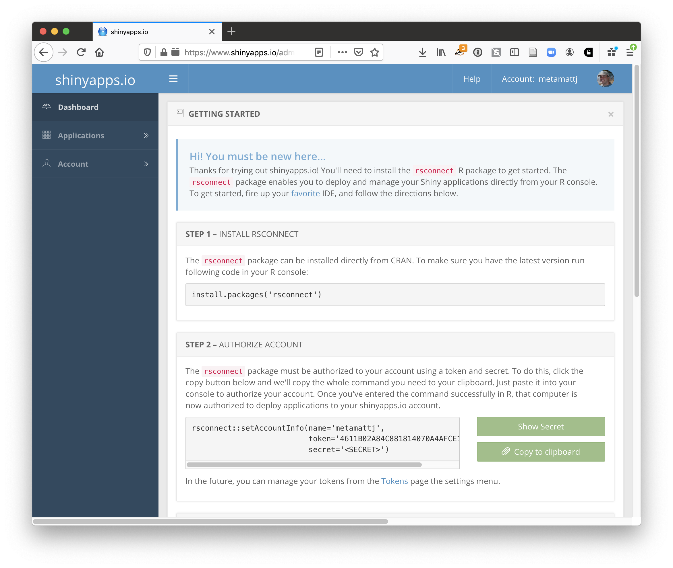
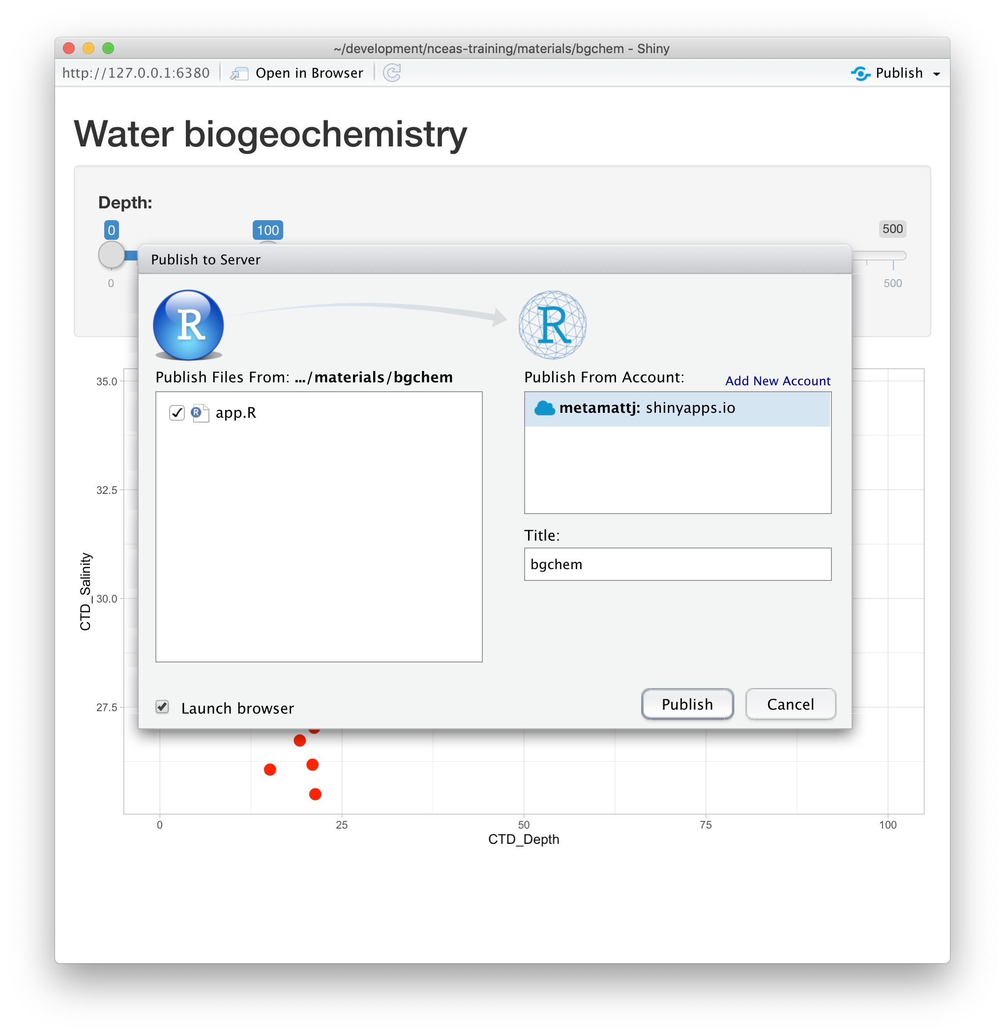
The easiest path is to create an account on shinyapps.io, and then configure RStudio to use that account for publishing. Instructions for enabling your local RStudio to publish to your account are displayed when you first log into shinyapps.io:
Once your account is configured locally, you can simply use the Publish button from the application window in RStudio, and your app will be live before you know it!