from pystac_client import Client
uri = 'https://earth-search.aws.element84.com/v1'
catalog = Client.open(uri)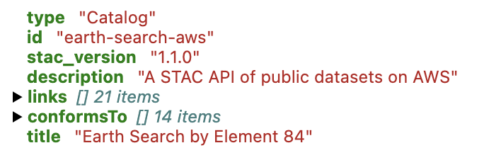
catalog17 Navigating the Cloud-scale Data Landscape
17.1 Learning Objectives
- Review the big picture of computational challenges in large-scale data analysis
- Recap various workshop technologies and how they all fit together
- Learn about cloud optimized data formats and access patterns
- Consider the present and future of cloud-native geospatial data
17.2 Introduction
This course has focused on scalable computing in the Arctic domain. In a nutshell, that means going big with our computing and data processing, and being equipped to deal with the challenges that arise when scaling up. But what exactly is it that can be big, what problems arise as a consequence, and what are the corresponding solutions? We’ve talked about how we can run into bottlenecks in CPU, memory, I/O, and network, but let’s step back and consider two major and distinct types of scaling challenges:
If your fundamental challenge is task volume, then aside from speeding up computation by using faster processors and/or faster algorithms, the natural solution (when permitted by the structure of the problem) is to transition to parallel processing, spreading tasks out across multiple cores, processors, and/or nodes. We’ve covered approaches to this using Python’s multithreading and multiprocessing capabilities, along with Parsl as a full-fledged parallel programming library.
If your fundamental challenge is data volume, then barring budget and means to sufficiently scale up your memory and storage capacity, the solution in one form or another is to split the data into pieces, working with each piece in turn. Interestingly, by decomposing a dataset into many small parts to act on independently, we often end up with a task architecture amenable to parallelization, allowing us to not only overcome the data volume problem but also reduce our task duration! This is one of the benefits we get from working with data-centric parallelization frameworks like Dask, with its distributed dataframes and arrays.
In the remainder of this chapter, we will primarily focus on the data volume challenge, in particular exploring how different decisions about data storage formats and layouts enable (or constrain) us as we attempt to work with data at large scale. We’ll formalize a couple of concepts we’ve alluded to throughout the course, introduce a few new technologies, and characterize the current state of best practice – with caveat that this is an evolving area!
17.3 Cloud optimized data
As we’ve seen, when it comes to global and even regional environmental phenomena observed using some form of remote-sensing technology, much of our data is now cloud-scale. In the most basic sense, this means many datasets – and certainly relevant collections of datasets that you might want to analyze together – no longer fit in local storage. So instead we put it in the massive, “infinitely” scalable cloud, where it is distributed across potentially many networked storage backends.
Practically speaking, accessing data in the cloud means using HTTP to request and receive data. Compared with traditional local storage, each read operation is much, much slower using HTTP over the internet than when reading a file on a local storage device, and the throughput (i.e., the number of bytes you can move per second) is much lower. Although we can’t change these basic differences, we can optimize our data to reduce their impact. We’ll talk about how in a moment. But first consider two other cloud-centric developments over the past handful of years:
- Video over the web. Millions (if not billions) of users consume multidimensional array data every day over the web, streaming video from services like YouTube, Netflix, Twitch, TikTok, and many other providers. Data access is fast, and at any given moment, our phones, TVs, and other devices are requesting and receiving just the small chunks of data they need.
- Web-scale, web-enabled databases. In the Zarr section, we marveled at our ability to quickly pull a tiny bit of data from a multi-terabyte data store in the cloud. But consider that we do this kind of thing all the time every day when we browse the web and use all manner of web services (either directly or indirectly): we request and receive small bits of data from what are often large, distributed data stores, powered by fast, modern database and database-like systems sitting behind web APIs.
Accessing and manipulating data from massive satellite product collections and other large environmental data arrays isn’t exactly the same problem, but it has some common attributes. Indeed, the cloud-native geospatial vision is to be able to provision and process big environmental geospatial data in similarly convenient and performant ways, using a combination of optimized storage architecture and matching optimized client-side technologies for working with that data. .
17.3.1 Cloud Optimized GeoTIFFs (COGs)
As we’ve discussed elsewhere in this course, geospatial rasters are a specialization of multi-dimensional arrays. First of all, they are inherently 2-dimensional, with dimensions corresponding to a geospatial coordinate system. Conceptually, we may have additional dimensions insofar as a “complete” raster data set may involve a set of rasters at different dates and times (temporal dimension), or corresponding to different spectral bands. Nevertheless, the standard paradigm is to treat these as a collection of 2D arrays (potentially stored within a single file), and leave it up to users to combine them as needed.
Today, best practice is to store geospatial rasters as Cloud Optimized GeoTIFFs, known as COGs. COGs are a relative newcomer among raster file formats. They first emerged in the mid-2010s, and were approved as an official standard of the Open Geospatial Consortium (OGC) in 2023. However, COGs are GeoTIFFs, which have been around since the 1990s, and GeoTIFFs are TIFFs, which date back to the 1980s. Let’s work our way through this lineage.
First we have the original TIFF format, which stands for Tagged Image File Format. Although we often think of TIFFs as image files, they’re actually file containers for images, insofar as a single TIFF file can store multiple raster images. In brief, TIFF have a file header - i.e., metadata - encoded in the bytes at the beginning of the file. Among other things, this header points to another batch of metadata (called an image file directory, or IFD) for a first image. This IFD contains information about where the image bytes themselves are located in the file, and also points to the IFD of a second image (if there is one), and so on. True to its name, TIFFs internally rely on so-called tags - simple data structures that store various attributes and properties - to capture information clients need to properly interpret and render the contained images. TIFFs also rely heavily on internal compression of the image data, using one of a few well-known lossless compression algorithms.
Next we have GeoTIFFs. GeoTIFFs are simply TIFFs with special tags that store geospatial information: how the image bounds relate to locations on the earth, coordinate reference system, datum, ellipsoid, projection. That’s about all there is to it.
Finally we have COGs. COGs are GeoTIFFs that following some specific conventions, none of which are required by the GeoTIFF standard itself, but all of which are compliant with it:
Metadata up front
All IFD bytes (i.e., the metadata for all contained images) are laid out sequentially at the beginning of the file, after the standard TIFF header. Readers don’t need to follow a chain of offsets to discover what the TIFF contains or where images are located in the file; they simply need to read a sufficiently large number of initial bytes.
Tiled data
The main raster data is broken into tiles (i.e., rectangular chunks) which are each individually compressed, and all stored in a particular sequential order. Tiling means individual raster values from nearby pixels tend to be close to each other in the file, indeed usually within the same compressed tile.
Overviews
A set of overviews (lower resolution tile pyramids) are computed from the main full resolution data and stored in the file, again following a tiling scheme and arranged in order. This allows clients to load a lower resolution version of the data when appropriate, without needing to read the full resolution data itself.
To reiterate, all of these are just restrictions on the GeoTIFF format, so a COG is a GeoTIFF. However, because of its deliberate design, clients can access relevant spatial subsets of a (potentially very large) raster by making just a few reads of discrete portions of the file. This is hugely important when accessing the data over HTTP – hence the “cloud optimized” moniker - because each HTTP read operation is far more time-consuming than the same corresponding read would be for a local disk read. Provided the data is hosted on a web server that accepts range requests for specific sections of a file rather than returning the entire file, we can access relevant chunks of data in a targeted and efficient manner.
Here is a rough sketch of what happens when a user wants data from a COG for some specific geographic area at 100m resolution, which we’ll assume is coarser than the full resolution in a COG. First the client makes an initial HTTP range request large enough to capture all metadata in most cases, e.g. the first 16 kilobytes of the file. This provides enough information to understand the file structure, georeferencing information, internal tile structure including overviews, and byte offsets to all overview and tile indexes. The client is then able to make precise HTTP range requests for the specific bytes needed for any particular desired subset of the image at a particular resolution (either full or reduced), by converting the geographic coordinates of the desired bounding box into pixel coordinates, then identifying which tile(s) in the COG intersect with the area of interest, then determining the associated byte ranges of the tile(s) based on the metadata read in the first step. And the best part is that “client” here refers to the underlying software, which takes care of all of the details. As a user, typically all you need to do is specify the file location, area of interest, and desired overview level (if relevant)!
17.3.2 Cloud-optimized data principles
How do we generalize the cloud-friendly features of COGs? It really comes down to two things:
The first is consolidating metadata and making it available “up front”. A consumer should be able to start by reading metadata only, ideally getting all of the essential metadata in one single read operation, without knowing anything else. This metadata should be sufficient for the client to determine not only what the dataset contains, but also exactly where to go to get any specific subset(s) of the overall available data.
The second is storing data in chunks, each of which can be accessed independently. Equal parts art and science, chunks should be reasonably sized – not too big, not too small – with chunk configuration (shape) optimized for expected usage patterns. This enables a client interested in a subset of data to retrieve the relevant data without receiving too much additional unwanted data. In addition, chunk layout should be such that, under expected common usage patterns, proximal chunks are more likely to be requested together. On average, this will reduce the number of separate read requests a client must issue to retrieve and piece together any particular desired data subset.
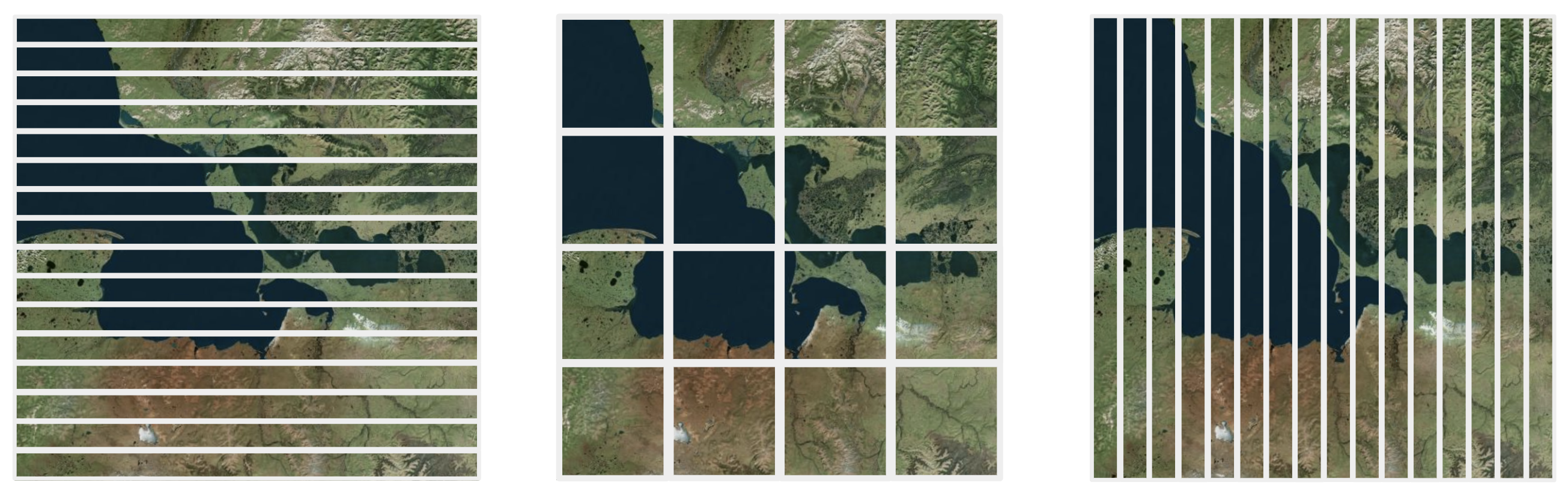
For example, in the image above depicting a simple 2D spatial raster dataset, consider three alternative chunking patterns. The approach on the left stores data together that share the same latitude, whereas the approach on the right stores data together that share the same longitude. In each case, values that are nearby but in the orthogonal direction will be split across multiple chunks, which is not ideal. Meanwhile, the square tile approach in the middle – consistent with the COG format specification – strikes a healthy balance, and overall is more effective at storing together data that are spatially proximal in any given direction. Now imagine a stack of such rasters corresponding to data collected over time – in other words, a 3D array dataset with a time dimension. The same principle holds in general: cubes will ensure that data that are proximal in both space and time will be stored in the same chunk, and are probably the safest bet. However, an alternative strategy may be preferable if, for example, the expected dominant use case is spatial analysis (consider storing tiles that are spatially broad but are shallower in the temporal dimension) or time-series analysis (consider storing tiles that are spatially narrow but are longer in the time dimension).
In addition, chunks should almost certainly be compressed with a suitable compression algorithm. Compression incurs some additional compute time for decompression, but with a net benefit because it reduces the total number of bytes transferred over the relatively slow network connections we experience in the cloud setting.
Together, these characteristics enable clients to efficiently (i.e., with a small number of read operations transferring minimal unwanted data) execute partial reads of data, and furthermore to speed things up by doing parallel reads of distinct sections of data.
To reiterate what we discussed in the COGs section, this is all deliberately designed to work well with HTTP range requests, a mechanism whereby clients can request specific byte ranges of a web-accessible resource. Through the combination of a smart chunk layout on one hand, with metadata up front on other hand, clients can quickly determine where to get data of interest, and then retrieve efficiently via HTTP range requests.
17.3.3 Zarr, revisited
Now that we understand what cloud optimized data formats are all about, let’s go back and revisit Zarr. Is it cloud friendly?
- Metadata up front. In Zarr stores, we expose metadata through external JSON files. Clients start by reading the metadata to determine where relevant data chunks live. Moreover, Zarr supports creation of consolidated metadata, whereby the metadata for all groups and arrays in a given Zarr store is packaged into a single metadata file in the root of the store, so that clients can access all of this information in a single read.
- Chunked data. Indeed, this is foundational to Zarr. Recall that Zarr is a storage specification for chunked, compressed N-dimensional arrays. Moreover, these chunks can be store in various ways – not only in memory and in conventional disk-based file systems, but also in cloud-based object storage such as Google Cloud Storage, Amazon S3, and Azure Blob Storage.
So by these criteria, yes, Zarr is certainly a cloud-friendly format!
But wait, there’s more! As of early 2025 with its V3 release, Zarr has introduced an important new cabilility around sharding, which controls how chunks are allocated to files. Previously, each chunk was compressed and stored as a separate file, but now multiple compressed chunks can be stored in the same file (referred to as a “shard”). In other words, the choice of how to break the data into separately compressed and addressable subsets is now decoupled from the choice of how to break the data into separate files; a massive dataset can be segmented into a very large number of small chunks without necessarily creating a correspondingly large number of small individual files, which can cause problems in certain contexts. In some sense, this allows a Zarr store to behave a little more like a COG, with its many small, addressable tiles contained in a single file.
17.3.4 Cloud-optimized netCDF files?
What about all those netCDF files out in the wild? Although one option would be to convert these into a cloud optimized format like Zarr, it turns out there’s another approach that can work well. Especially in cases where the netCDF file already has well-designed internal chunking and sensible compression – both features already supported by the specification – the only other thing we really need is relevant metadata up front. We can achieve this by creating Zarr-like metadata that fully describes the data in an external JSON file, pointing at byte-addressed segments of the relevant netCDF file(s) rather than independent data files/objects stored in native Zarr format. Sometimes referred to as virtual Zarr stores, these can be created using libraries such as kerchunk and VirtualiZarr.
If the original source netCDF files are not effectively chunked (internally) for your relevant analysis use cases, virtual Zarr stores aren’t going to help much. In that case, it may be better to convert the data (or the desired subset of data) into a proper Zarr store with better chunking. However, in other cases, the virtual Zarr approach can work quite well, typically yielding more or less equivalent read performance between the two approaches.
17.4 SpatioTemporal Asset Catalogs (STAC)
Today we have data, data, everywhere, made available by many providers in multiple formats. Across this landscape, how can we effectively find data of interest for a particular place and time, and quickly understand how to access, ingest, and use each individual data resource? Historically, organizations publishing data over the web have each used their own ad hoc methods for documenting and cataloging available files. For example, recall in the Zarr chapter when we downloaded and searched through a large CSV file to find paths to relevant CMIP6 datasets. Wouldn’t it be nice if all providers agreed to a common cataloging approach, so we didn’t have to figure out the idiosyncrasies of each scheme? This is exactly the problem that STAC is designed to solve.
STAC is a specification for describing spatiotemporal data assets, intended to facilitate the search and discovery of relevant data collected at some place and time on Earth, especially based on spatial and/or temporal queries of interest.
![]()
To work with STAC, you need to be comfortable with the following terms:
| STAC term | Description |
|---|---|
| Asset | A file representing information about the Earth, captured at some place and time |
| Item | A document describing one or more assets associated with a given place and time, with metadata describing that place (as a GeoJSON feature), time, and various other properties |
| Collection | A document describing a set of items and/or child collections, with metadata describing their collective spatiotemporal extent, and other various properties |
| Catalog | A grouping of items, collections, and/or other child catalogs |
| Link | A reference to a related resource either in the catalog (e.g., related items) or outside the catalog (e.g. documentation) |
STAC catalogs come in two variants. The simpler form is a static catalog, achieved by simply publishing STAC-compliant JSON files on the web. Clients can read these files, walk through the linked information to identify and explore component collections and items, and ultimately get to the associated data via asset links.
The second form is a dynamic API. This requires more setup by the catalog publisher, including provisioning of an API server, but it enables more powerful catalog interactions such as dynamic search.
Let’s take a quick peek at how we can use Python, including the pystac-client library, to navigate a STAC catalog and ultimately retrieve some data, borrowing from this online tutorial. We’ll use Earth Search by Element 84, a STAC catalog implemented as a dynamic API. Before we dive into the code, you may want to have a look at the web-based catalog browser, which can be useful for interactive exploration.
In this book we’ve simply included static screenshots of the output, but in a Jupyter notebook or similar interactive environment, you would be able to expand various sections and drill into the hierarchical depths of the returned information.
First let’s connect to the top-level catalog.
Now we’ll see what collections are stored at the Catalog level.
collection_list = list(catalog.get_collections())
print(f"Catalog contains {len(collection_list)} collections")
for collection in collection_list:
    print(f'- [{collection.id}] {collection.title}')
Catalog contains 9 collections
- [sentinel-2-pre-c1-l2a] Sentinel-2 Pre-Collection 1 Level-2A
- [cop-dem-glo-30] Copernicus DEM GLO-30
- [naip] NAIP: National Agriculture Imagery Program
- [cop-dem-glo-90] Copernicus DEM GLO-90
- [landsat-c2-l2] Landsat Collection 2 Level-2
- [sentinel-2-l2a] Sentinel-2 Level-2A
- [sentinel-2-l1c] Sentinel-2 Level-1C
- [sentinel-2-c1-l2a] Sentinel-2 Collection 1 Level-2A
- [sentinel-1-grd] Sentinel-1 Level-1C Ground Range Detected (GRD)Let’s dive into the sentinel-2-l2a collection.
In the returned widget, look at some of the details. Especially take note of the extent field, which contains information about the spatial and temporal coverage of this collection. This is central to STAC! In this case, the collection has global bounds, with a time period beginning in June 2015 and continuing today.
sentinel_collection_id = 'sentinel-2-l2a'
catalog.get_collection(sentinel_collection_id)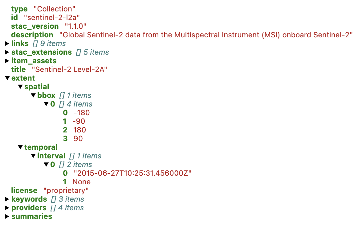
What does this collection contain? For starters, how big is the collection, in terms of the number of items?
Tip
Here’s a trick to get a total item count: We’ll do a search on the catalog, specifically referencing the collection of interest, but otherwise not providing any query constraints. Importantly, we’ll also tell this method not to return any items. Then we’ll invoke the returned object’s matched() method, helpfully reporting the total count of “matched” items – which in this case is the total count of items in the collection.
n = catalog.search(collections=[sentinel_collection_id], max_items=0).matched()
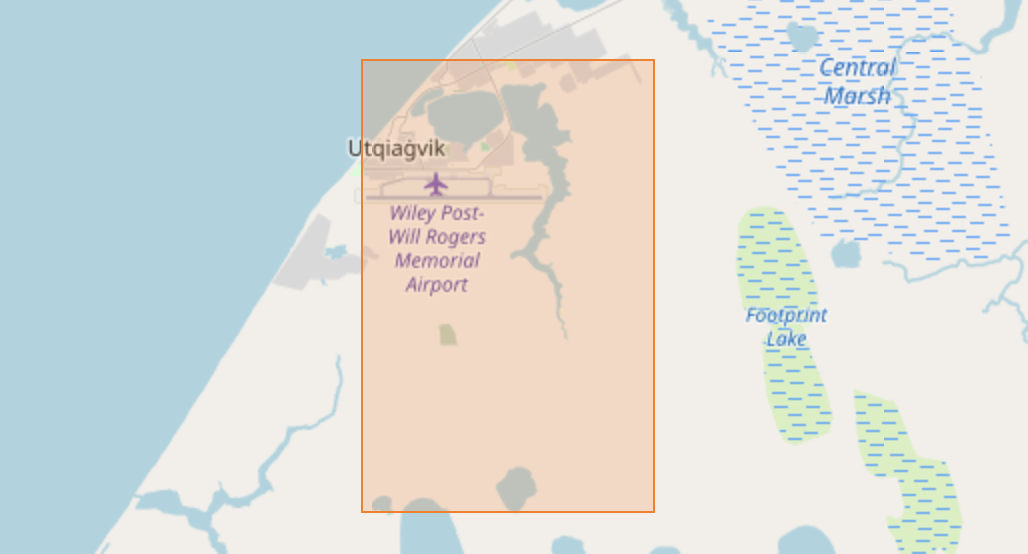
print(f'Found {n:,} items in the {sentinel_collection_id} collection')Found 39,950,465 items in the sentinel-2-l2a collectionWow, that’s a lot! We certainly don’t want to pull down metadata for all of these items. To retrieve only a subset of interest, we’ll go back to the catalog.search() method, but this time providing some significant restrictions on what we want. In particular, we’ll limit by temporal extent using a date range spanning a few months, and by geographic extent using a (manually created) bounding box corresponding to a small area near Utqiagvik.
east, west, north, south = -156.7, -156.8, 71.3, 71.25
bbox_utqiagvik = [west, south, east, north]

item_collection = catalog.search(
    collections=[sentinel_collection_id],
    bbox=bbox_utqiagvik,
    datetime="2020-03-01/2020-06-01"
).item_collection()

print(f'Returned {len(item_collection)} items')
item_collection.items[0]
Returned 148 items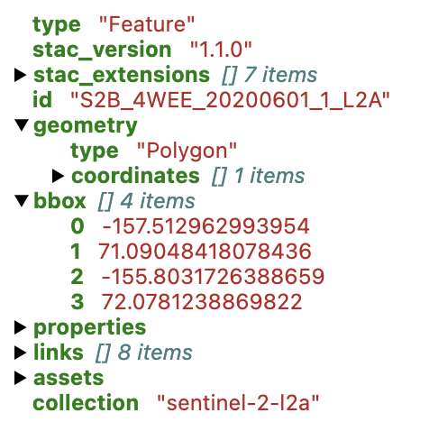
The specific geographic extent of each associated item is recorded in the geometry and bbox fields, and the temporal information is stored in a datetime field under properties (not shown above).
Remember, a STAC item is still just a catalog entry, not the underlying data or other artifact itself. STAC doesn’t actually store data, but like any useful catalog, it tells you where to find it. In STAC parlance, the “things” it refers to are called assets, which “belong” to an item. An item can refer to many assets. You can see them under the assets entry in the catalog visualizer above, or access them in a dictionary-like way using the assets accessor on the item.
In this case, each item references multiple assets. Let’s look at one particular asset called nir, which contains the near infrared reflectance band associated with this Sentinel scene.
item_collection.items[0].assets['nir']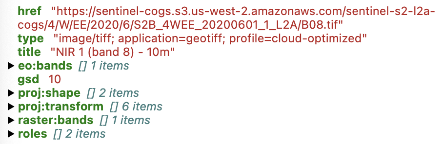
From the information above, we can see that the nir reflectance data artifact corresponding to this asset is stored as a cloud optimized GeoTIFF in AWS S3 storage. We can take the individual COG URL and throw it in this cool interactive COG web mapper site, and of course we could load this data into Python as a distributed dask array using rasterio or rioxarray, depending on our preference.
# use rioxarray, which implicitly uses rasterio + xarray
import rioxarray
href = "https://sentinel-cogs.s3.us-west-2.amazonaws.com/sentinel-s2-l2a-cogs/4/W/EE/2020/6/S2B_4WEE_20200601_1_L2A/B08.tif"
rx_nir = rioxarray.open_rasterio(href, chunks={})
Lastly, what if we wanted to assemble a bunch of spatially aligned COGs for multiple different dates? We could do it manually by looping over all of the items … or we could save time and use stackstac! The stackstac library provides a convenient way to wrangle a set of STAC items into a single xarray array, using lazy loading and dask under the hood. Here let’s just take the first 10 items by date, focus on the same nir asset as above, again provide the bounding box – which in this case will be used to subset (i.e., clip) the data rather than simply retrieving overlapping items, which is what our earlier STAC search did – and even transform the data on the fly to WGS84.
import stackstac

east, west, north, south = -156.7, -156.8, 71.3, 71.25
stack = stackstac.stack(
    item_collection[:10],
    assets=['nir'],
    bounds_latlon=[west, south, east, north],
    epsg=4326
)
stack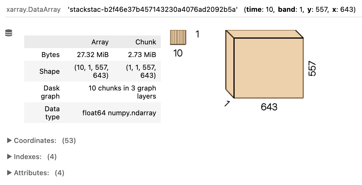
Finally, let’s do a quick plot faceted by time, showing the 6 clipped rasters with data from among the set of items we pulled.
stack \
    .isel(time=slice(0, 6)) \
    .squeeze() \
    .plot.imshow(col="time", col_wrap=3, robust=True)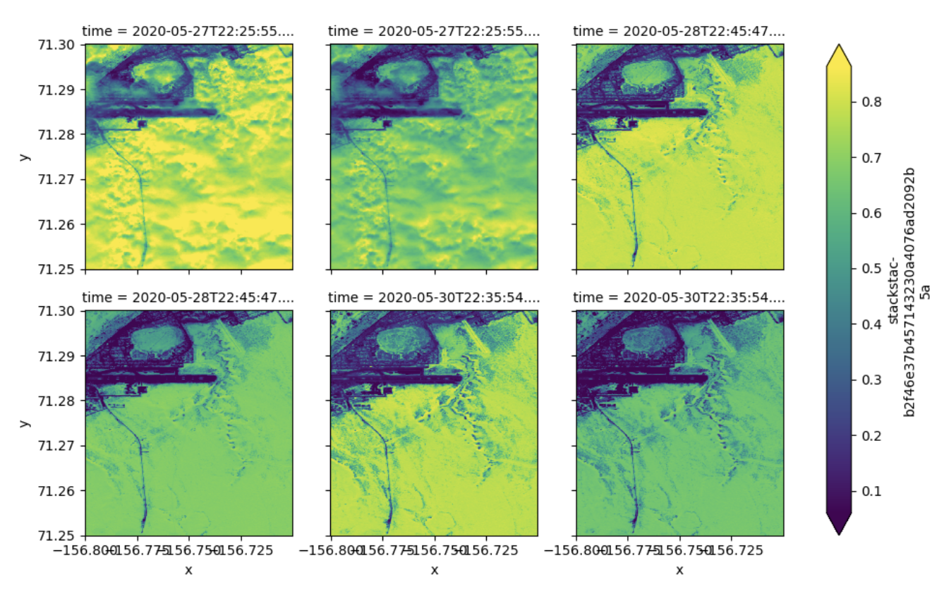
There we have it! With the help of the STAC specification and associated libraries for enabling us to seamlessly assemble a local dataset from across many files, and the COG specification and associated libraries for enabling us to seamlessly pull out small portions of the data from within each file, we can very rapidly and efficiently piece together our own custom multidimensional data array from a large collection of data resources that themselves be arbitrarily organized with respect to our specific use case.
Interested in learning more about STAC? If so, head over to the STAC Index, an online resource listing many published STAC catalogs, along with various related software and tooling.
17.5 Making sense of the menagerie
Consider this diagram showing data laid out in various ways, all available for you to find, access, retrieve, and ultimately manipulate from your chosen compute platform, whether it’s a single (physical or virtual) machine running some number of CPUs each with some number of cores, or a distributed cluster of many such machines.
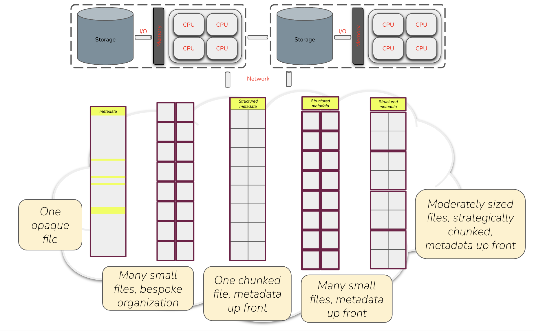
Moving left to right across the five generalized data architectures depicted above, the first reflects our legacy world of irregularly structured netCDF and GeoTIFF files – historically successful and efficiently used in local storage, but often suboptimal at cloud scale. The second represents simple, ad hoc approaches to splitting larger data into smaller files, thrown somewhere on a network-accessible server, but without efficiently readable overarching metadata and without any optimal structure. The next two represent cloud optimized approaches, with data split into addressable units described by up-front metadata that clients can use to efficiently access the data. The first of these resembles a COG (one file containing many addressable pieces), while the second resembles a traditional Zarr store (many addressable pieces as separate files). This highlights two different approaches that you’ve encountered in this courses:
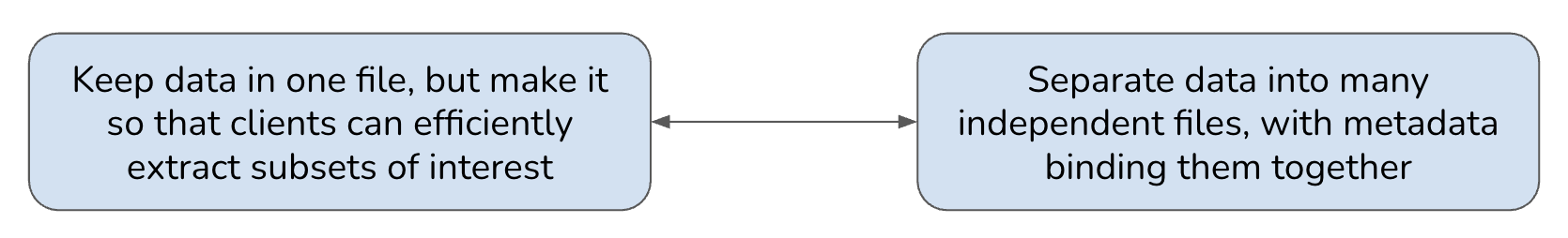
Which is better? The likely answer is … both! Indeed, the community seems to be converging on a hybrid model whereby we use a combination of chunking (splitting the data into sections) and sharding (storing multiple chunks together) to achieve the right balance between not having too many individual files/objects (which would be the case if we chunked without sharding), and not having individual files/objects that are too big (which would be the case if we put all chunks into one shard). This decision can be made separately for any given data collection, and its complexity can be shielded from users through the use of external metadata – whether as Zarr metadata or STAC catalogs – that allows clients to issue data requests that “just work” regardless of the underlying implementation details.
As a final takeaway, insofar as there’s a community consensus around the best approaches for managing data today, it probably looks something like this:
- COG and STAC, working together, as the go-to approach for storing and provisioning related geospatial raster datasets in the cloud
- Zarr stores (with intelligent chunking and sharding), potentially referenced by STAC catalogs, as the go-to approach for storing and provisioning multidimensional Earth array data in the cloud
- Virtual Zarr stores, again potentially in conjunction with STAC catalogs, as a cost-effective approach for cloud-enabling many legacy data holdings in netCDF format
If you’re making large scale data available yourself, this is probably the way to go. If you’re purely a data consumer, you’re not likely to have much influence over how the data you need is organized and provisioned, but being comfortable with the above technologies will likely set you up well for the future.
17.6 Summary
We’ve covered a diverse set of topics in this chapter and in this course. The goal was not to impart deep expertise in any one area, but rather to survey a handful of useful tools and illustrate some general principles that will ease your adoption of cloud-scale compute and data analysis technologies – especially as a consumer, and maybe even occasional provider, of large, multidimensional environmental datasets.
You should now have a better appreciation for the following questions, why they are important to ask, and how you might go about answering them:
- What kind of data do I have? If array data, am I dealing with geospatial rasters or generalized n-dimensional arrays?
- What is the (existing) file format, and what tradeoffs does that create for me when working with the data? Could I benefit from converting to a different format, if feasible?
- Is the data local or remote? If remote, where exactly is it located? Can I practically retrieve and store it locally?
- In either case, can I fit the data in memory when working with it?
- If not, is the data set up to allow efficient access to (or splitting into) individual subsets?
- If so, is the subsetting scheme well-suited to my expected access patterns?
- Assuming I can get (subsets of) the data, can I process separate pieces in parallel?
- If so, what are my options for distributing the processing of these subsets across workers, and how can I determine whether it’s helping me get work done faster?
If you want to check your understanding further and get inspired to think more about the challenges of and solutions to cloud-scale processing and analysis, have a look at this list of cloud-data antipatterns published by the Earth Science Information Partners (ESIP) Cloud Computing Cluster (CCC). Armed with the information presented in this chapter and in earlier parts of this course, most of the items on this list should make sense to you now, at least at a high level: why these are considered antipatterns (i.e., suboptimal approaches), and how the various tools, technologies, and approaches we’ve covered seek to avoid this problems.