1 Welcome and Introductions

This course is one of three that we are currently offering, covering fundamentals of open data sharing, reproducible research, ethical data use and reuse, and scalable computing for reusing large data sets.

1.1 Introduction to the Arctic Data Center and NSF Standards and Policies

1.1.1 Learning Objectives

In this lesson, we will discuss:

The mission and structure of the Arctic Data Center
How the Arctic Data Center supports the research community
About data policies from the NSF Arctic program

1.1.2 Arctic Data Center - History and Introduction

The Arctic Data Center is the primary data and software repository for the Arctic section of National Science Foundation’s Office of Polar Programs (NSF OPP).

We’re best known in the research community as a data archive – researchers upload their data to preserve it for the future and make it available for re-use. This isn’t the end of that data’s life, though. These data can then be downloaded for different analyses or synthesis projects. In addition to being a data discovery portal, we also offer top-notch tools, support services, and training opportunities. We also provide data rescue services.

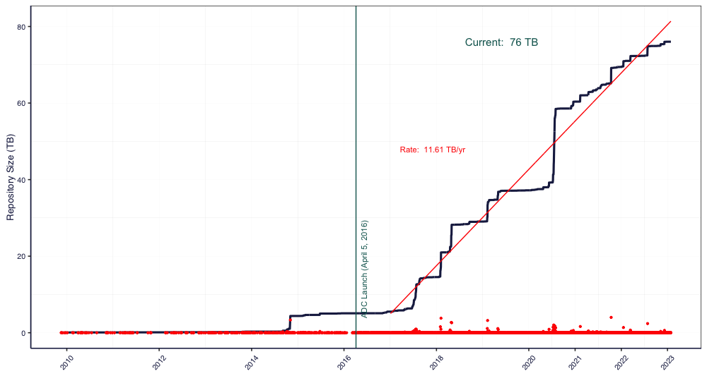
NSF has long had a commitment to data reuse and sharing. Since our start in 2016, we’ve grown substantially – from that original 4 TB of data from ACADIS to now over 76 TB at the start of 2023. In 2021 alone, we saw 16% growth in dataset count, and about 30% growth in data volume. This increase has come from advances in tools – both ours and of the scientific community, plus active community outreach and a strong culture of data preservation from NSF and from researchers. We plan to add more storage capacity in the coming months, as researchers are coming to us with datasets in the terabytes, and we’re excited to preserve these research products in our archive. We’re projecting our growth to be around several hundred TB this year, which has a big impact on processing time. Give us a heads up if you’re planning on having larger submissions so that we can work with you and be prepared for a large influx of data.

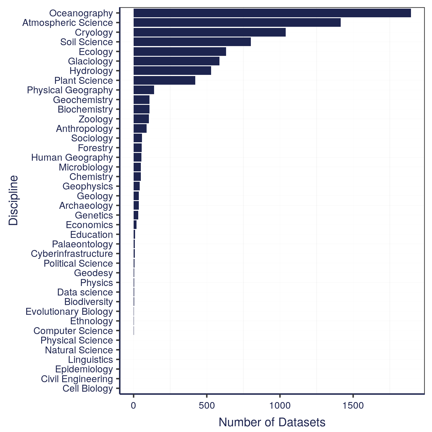
The data that we have in the Arctic Data Center comes from a wide variety of disciplines. These different programs within NSF all have different focuses – the Arctic Observing Network supports scientific and community-based observations of biodiversity, ecosystems, human societies, land, ice, marine and freshwater systems, and the atmosphere as well as their social, natural, and/or physical environments, so that encompasses a lot right there in just that one program. We’re also working on a way right now to classify the datasets by discipline, so keep an eye out for that coming soon.

Along with that diversity of disciplines comes a diversity of file types. The most common file type we have are image files in four different file types. Probably less than 200-300 of the datasets have the majority of those images – we have some large datasets that have image and/or audio files from drones. Most of those 6600+ datasets are tabular datasets. There’s a large diversity of data files, though, whether you want to look at remote sensing images, listen to passive acoustic audio files, or run applications – or something else entirely. We also cover a long period of time, at least by human standards. The data represented in our repository spans across centuries.

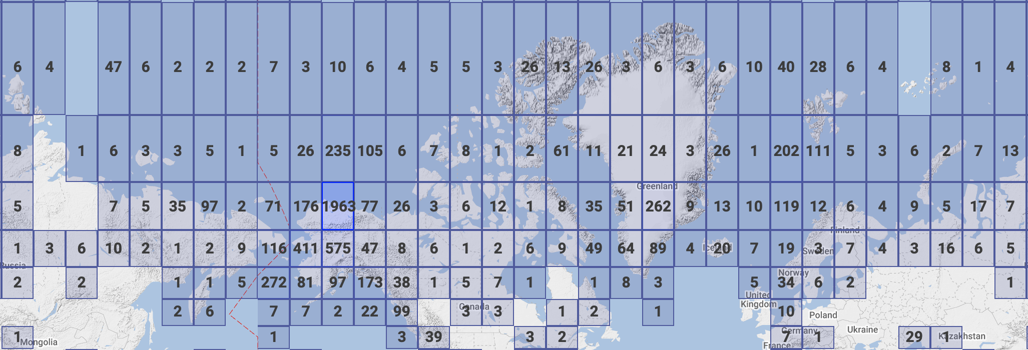
We also have data that spans the entire Arctic, as well as the sub-Arctic, regions.

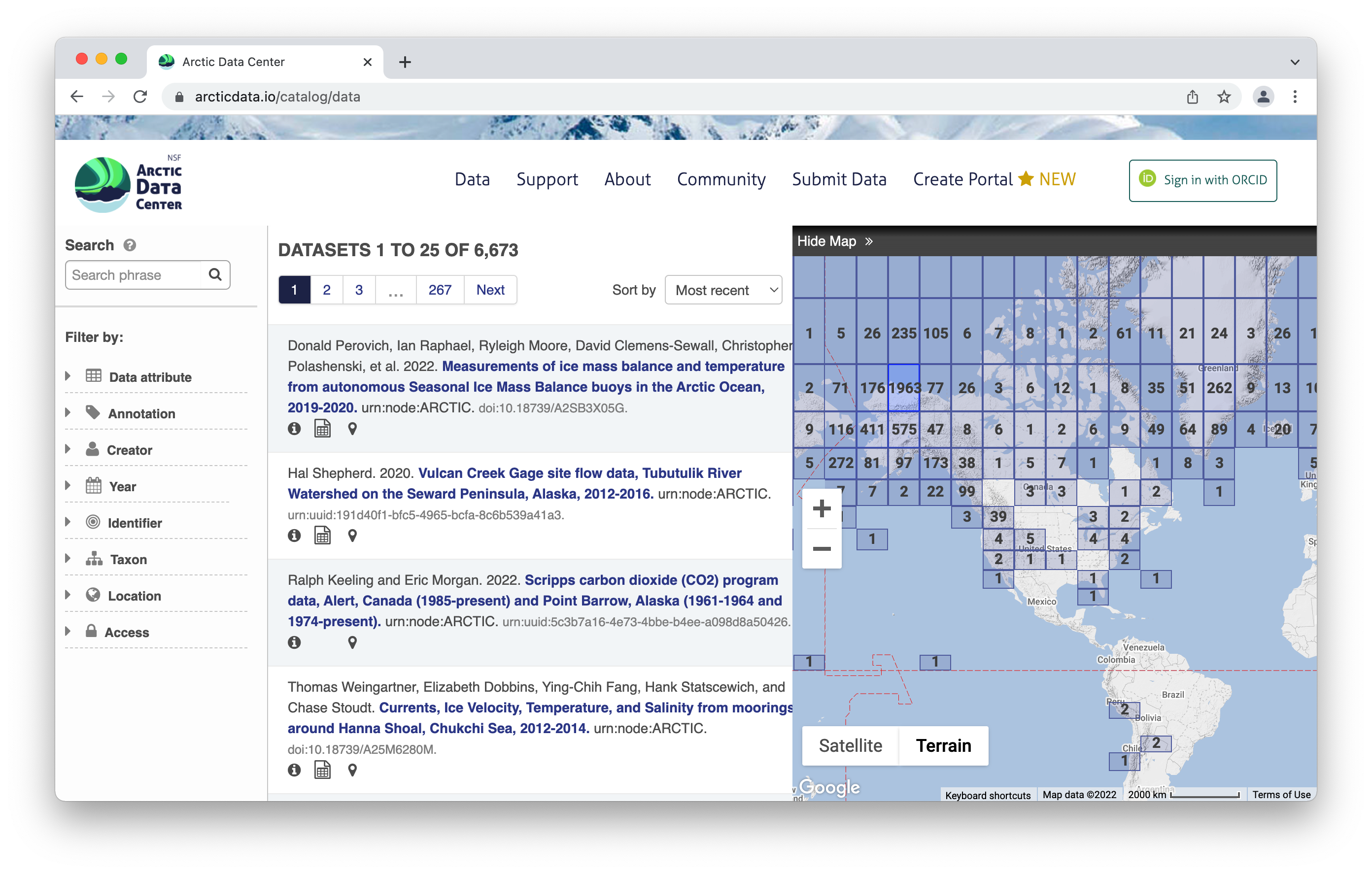
1.1.3 Data Discovery Portal

To browse the data catalog, navigate to arcticdata.io. Go to the top of the page and under data, go to search. Right now, you’re looking at the whole catalog. You can narrow your search down by the map area, a general search, or searching by an attribute.

Clicking on a dataset brings you to this page. You have the option to download all the files by clicking the green “Download All” button, which will zip together all the files in the dataset to your Downloads folder. You can also pick and choose to download just specific files.

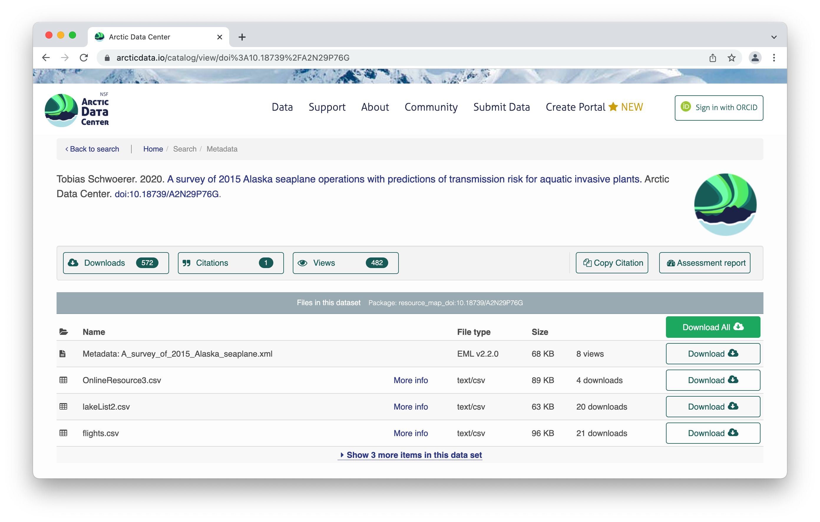
All the raw data is in open formats to make it easily accessible and compliant with FAIR principles – for example, tabular documents are in .csv (comma separated values) rather than Excel documents.

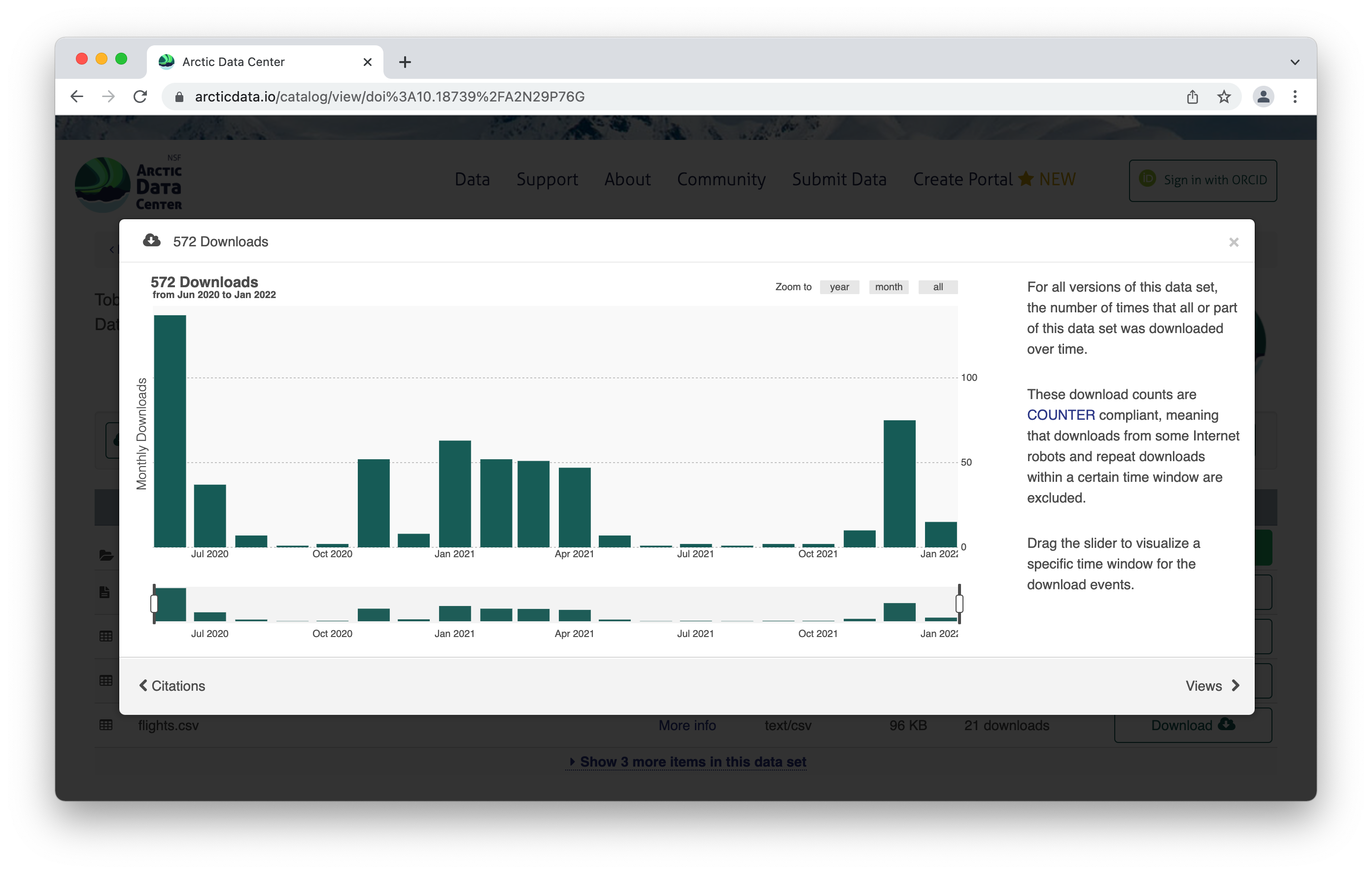
The metrics at the top give info about the number of citations with this data, the number of downloads, and the number of views. This is what it looks like when you click on the Downloads tab for more information.

Scroll down for more info about the dataset – abstract, keywords. Then you’ll see more info about the data itself. This shows the data with a description, as well as info about the attributes (or variables or parameters) that were measured. The green check mark indicates that those attributes have been annotated, which means the measurements have a precise definition to them. Scrolling further, we also see who collected the data, where they collected it, and when they collected it, as well as any funding information like a grant number. For biological data, there is the option to add taxa.

1.1.4 Tools and Infrastructure

Across all our services and partnership, we are strongly aligned with the community principles of making data FAIR (Findable, Accesible, Interoperable and Reusable).

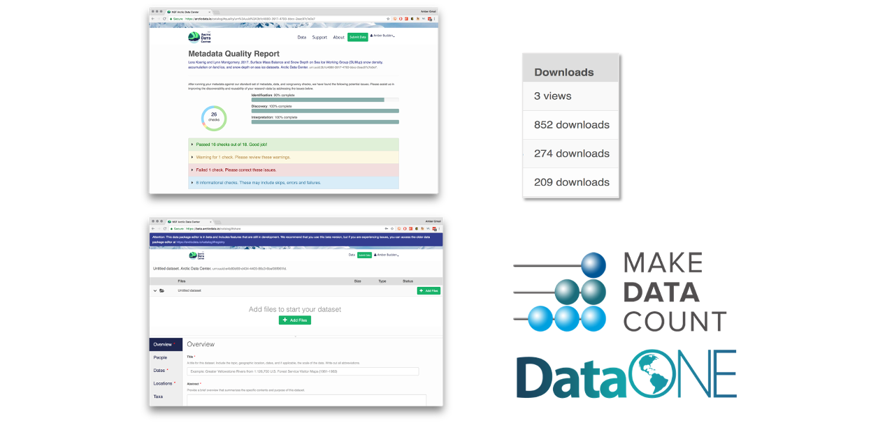
We have a number of tools available to submitters and researchers who are there to download data. We also partner with other organizations, like Make Data Count and DataONE, and leverage those partnerships to create a better data experience.

One of those tools is provenance tracking. With provenance tracking, users of the Arctic Data Center can see exactly what datasets led to what product, using the particular script that the researcher ran.

Another tool are our Metadata Quality Checks. We know that data quality is important for researchers to find datasets and to have trust in them to use them for another analysis. For every submitted dataset, the metadata is run through a quality check to increase the completeness of submitted metadata records. These checks are seen by the submitter as well as are available to those that view the data, which helps to increase knowledge of how complete their metadata is before submission. That way, the metadata that is uploaded to the Arctic Data Center is as complete as possible, and close to following the guideline of being understandable to any reasonable scientist.

1.1.5 Support Services

Metadata quality checks are the automatic way that we ensure quality of data in the repository, but the real quality and curation support is done by our curation team. The process by which data gets into the Arctic Data Center is iterative, meaning that our team works with the submitter to ensure good quality and completeness of data. When a submitter submits data, our team gets a notification and beings to evaluate the data for upload. They then go in and format it for input into the catalog, communicating back and forth with the researcher if anything is incomplete or not communicated well. This process can take anywhere from a few days or a few weeks, depending on the size of the dataset and how quickly the researcher gets back to us. Once that process has been completed, the dataset is published with a DOI (digital object identifier).

1.1.6 Training and Outreach

In addition to the tools and support services, we also interact with the community via trainings like this one and outreach events. We run workshops at conferences like the American Geophysical Union, Arctic Science Summit Week and others. We also run an intern and fellows program, and webinars with different organizations. We’re invested in helping the Arctic science community learn reproducible techniques, since it facilitates a more open culture of data sharing and reuse.

We strive to keep our fingers on the pulse of what researchers like yourselves are looking for in terms of support. We’re active on Twitter to share Arctic updates, data science updates, and specifically Arctic Data Center updates, but we’re also happy to feature new papers or successes that you all have had with working with the data. We can also take data science questions if you’re running into those in the course of your research, or how to make a quality data management plan. Follow us on Twitter and interact with us – we love to be involved in your research as it’s happening as well as after it’s completed.

1.1.7 Data Rescue

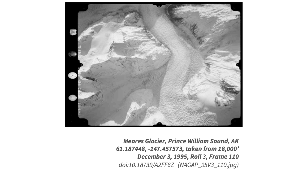
We also run data rescue operations. We digitiazed Autin Post’s collection of glacier photos that were taken from 1964 to 1997. There were 100,000+ files and almost 5 TB of data to ingest, and we reconstructed flight paths, digitized the images of his notes, and documented image metadata, including the camera specifications.

1.1.8 Who Must Submit

Projects that have to submit their data include all Arctic Research Opportunities through the NSF Office of Polar Programs. That data has to be uploaded within two years of collection. The Arctic Observing Network has a shorter timeline – their data products must be uploaded within 6 months of collection. Additionally, we have social science data, though that data often has special exceptions due to sensitive human subjects data. At the very least, the metadata has to be deposited with us.

Arctic Research Opportunities (ARC)

Complete metadata and all appropriate data and derived products
Within 2 years of collection or before the end of the award, whichever comes first

ARC Arctic Observation Network (AON)

Complete metadata and all data
Real-time data made public immediately
Within 6 months of collection

Arctic Social Sciences Program (ASSP)

NSF policies include special exceptions for ASSP and other awards that contain sensitive data
Human subjects, governed by an Institutional Review Board, ethically or legally sensitive, at risk of decontextualization
Metadata record that documents non-sensitive aspects of the project and data
- Title, Contact information, Abstract, Methods

For more complete information see our “Who Must Submit” webpage

Recognizing the importance of sensitive data handling and of ethical treatment of all data, the Arctic Data Center submission system provides the opportunity for researchers to document the ethical treatment of data and how collection is aligned with community principles (such as the CARE principles). Submitters may also tag the metadata according to community develop data sensitivity tags. We will go over these features in more detail shortly.

1.1.9 Summary

All the above informtion can be found on our website or if you need help, ask our support team at support@arcticdata.io or tweet us @arcticdatactr!

1.2 RStudio Setup

1.2.1 Learning Objectives

In this lesson, you will learn:

Creating an R project and how to organize your work in a project
Supplemental objective: How to make sure your local RStudio environment is set up for analysis
Supplemental objective: How to set up Git and GitHub

1.2.2 Logging into the RStudio server

To prevent us from spending most of this lesson troubleshooting the myriad of issues that can arise when setting up the R, RStudio, and git environments, we have chosen to have everyone work on a remote server with all of the software you need installed. We will be using a special kind of RStudio just for servers called RStudio Server. If you have never worked on a remote server before, you can think of it like working on a different computer via the internet. Note that the server has no knowledge of the files on your local filesystem, but it is easy to transfer files from the server to your local computer, and vice-versa, using the RStudio server interface.

Here are the instructions for logging in and getting set up:

Server Setup

You should have received an email prompting you to change your password for your server account. If you did not, please put up a post-it and someone will help you.

If you were able to successfully change your password, you can log in at: https://included-crab.nceas.ucsb.edu/

1.2.3 Why use an R project?

In this workshop, we are going to be using R project to organize our work. An R project is tied to a directory on your local computer, and makes organizing your work and collaborating with others easier.

The Big Idea: using an R project is a reproducible research best practice because it bundles all your work within a working directory. Consider your current data analysis workflow. Where do you import you data? Where do you clean and wrangle it? Where do you create graphs, and ultimately, a final report? Are you going back and forth between multiple software tools like Microsoft Excel, JMP, and Google Docs? An R project and the tools in R that we will talk about today will consolidate this process because it can all be done (and updated) in using one software tool, RStudio, and within one R project.

We are going to be doing nearly all of the work in this course in one R project.

Our version of RStudio Server allows you to share projects with others. Sharing your project with the instructors of the course will allow for them to jump into your session and type along with you, should you encounter an error you cannot fix.

Creating your project

In your RStudio server session, follow these steps to set up your shared project:

In the “File” menu, select “New Project”
Click “New Directory”
Click “New Project”
Under “Directory name” type: training_{USERNAME}, eg: training_do-linh
Leave “Create Project as subdirectory of:” set to ~
Click “Create Project”

Your RStudio should open your project automatically after creating it. One way to check this is by looking at the top right corner and checking for the project name.

1.2.4 Understand how to use paths and working directories

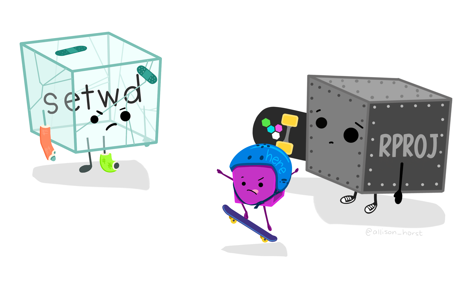
Artwork by Allison Horst. A cartoon of a cracked glass cube looking frustrated with casts on its arm and leg, with bandaids on it, containing “setwd,” looks on at a metal riveted cube labeled “R Proj” holding a skateboard looking sympathetic, and a smaller cube with a helmet on labeled “here” doing a trick on a skateboard.

Now that we have your project created (and notice we know it’s an R Project because we see a .Rproj file in our Files pane), let’s learn how to move in a project. We do this using paths.

There are two types of paths in computing: absolute paths and relative paths.

An absolute path always starts with the root of your file system and locates files from there. The absolute path to my project directory is: /home/do-linh/training_do-linh

Relative paths start from some location in your file system that is below the root. Relative paths are combined with the path of that location to locate files on your system. R (and some other languages like MATLAB) refer to the location where the relative path starts as our working directory.

RStudio projects automatically set the working directory to the directory of the project. This means that you can reference files from within the project without worrying about where the project directory itself is. If I want to read in a file from the data directory within my project, I can simply type read.csv("data/samples.csv") as opposed to read.csv("/home/do-linh/training_do-linh/data/samples.csv")

This is not only convenient for you, but also when working collaboratively. We will talk more about this later, but if Matt makes a copy of my R project that I have published on GitHub, and I am using relative paths, he can run my code exactly as I have written it, without going back and changing "/home/do-linh/training_do-linh/data/samples.csv" to "/home/jones/training_jones/data/samples.csv"

Note that once you start working in projects you should basically never need to run the setwd() command. If you are in the habit of doing this, stop and take a look at where and why you do it. Could leveraging the working directory concept of R projects eliminate this need? Almost definitely!

Similarly, think about how you work with absolute paths. Could you leverage the working directory of your R project to replace these with relative paths and make your code more portable? Probably!

1.2.5 Organizing your project

When starting a new research project, one of the first things I do is create an R project for it (just like we have here!). The next step is to then populate that project with relevant directories. There are many tools out there that can do this automatically. Some examples are rrtools or usethis::create_package(). The goal is to organize your project so that it is a compendium of your research. This means that the project has all of the digital parts needed to replicate your analysis, like code, figures, the manuscript, and data access.

There are lots of good examples out there of research compendia. Here is one from a friend of NCEAS, Carl Boettiger, which he put together for a paper he wrote.

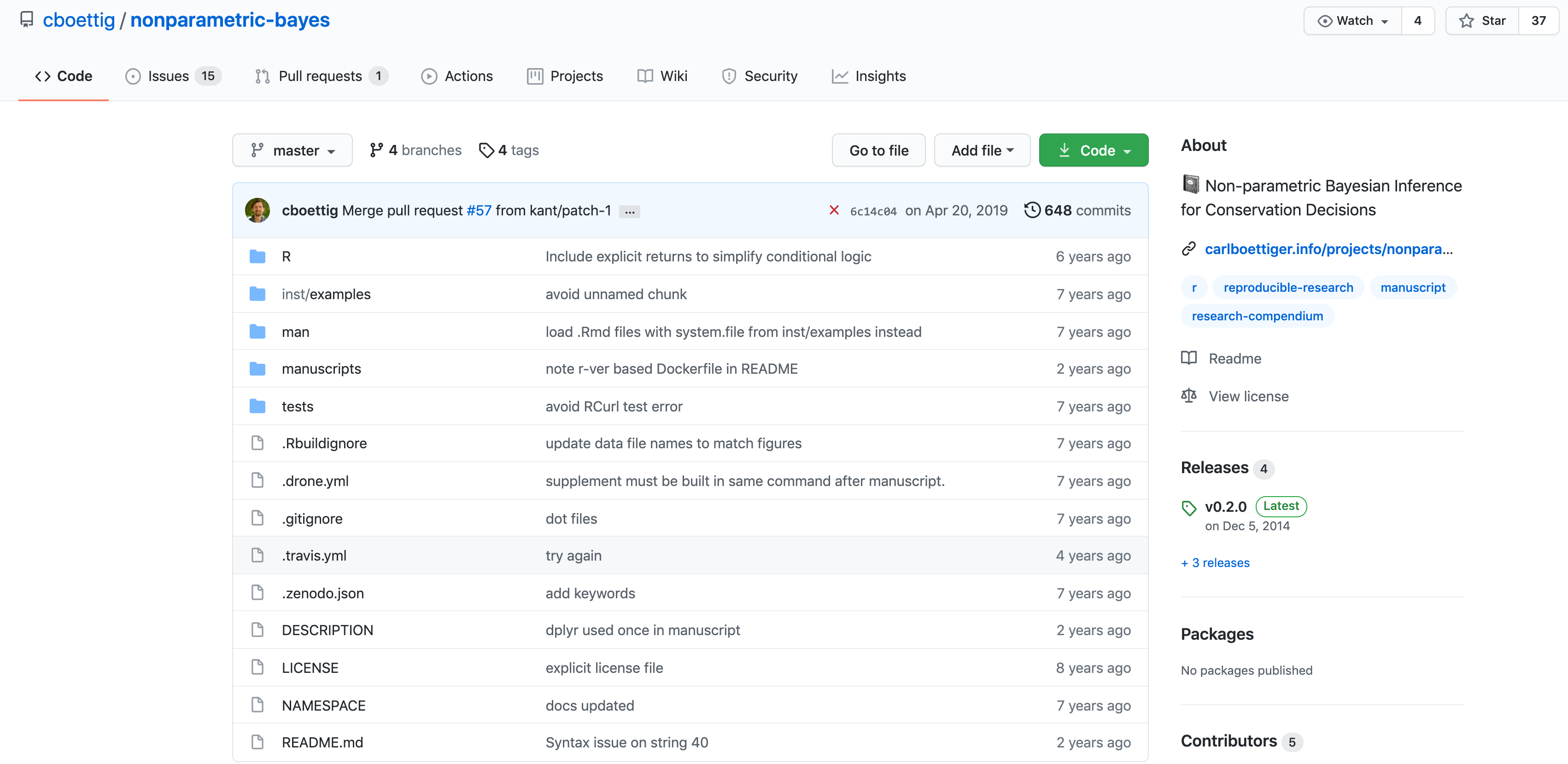
The complexity of this project reflects years of work. Perhaps more representative of the situation we are in at the start of our course is a project that looks like this one, which we have just started at NCEAS.

Currently, the only file in your project is your .Rproj file. Let’s add some directories and start a file folder structure. Some common directories are:

data: where we store our data (often contains subdirectories for raw, processed, and metadata data)
R: contains scripts for cleaning or wrangling, etc. (some find this name misleading if their work has other scripts beyond the R programming language, in which case they call this directory scripts)
plots or figs: generated plots, graphs, and figures
doc: summaries or reports of analysis or other relevant project information

Directory organization will vary from project to project, but the ultimate goal is to create a well organized project for both reproducibility and collaboration.

1.2.6 Summary

organize your research into projects using R projects
use R project working directories instead of setwd()
use relative paths from those working directories, not absolute paths
structure your R project as a compendium

1.2.7 Supplemental Objectives

1.2.7.1 Preparing to work in RStudio

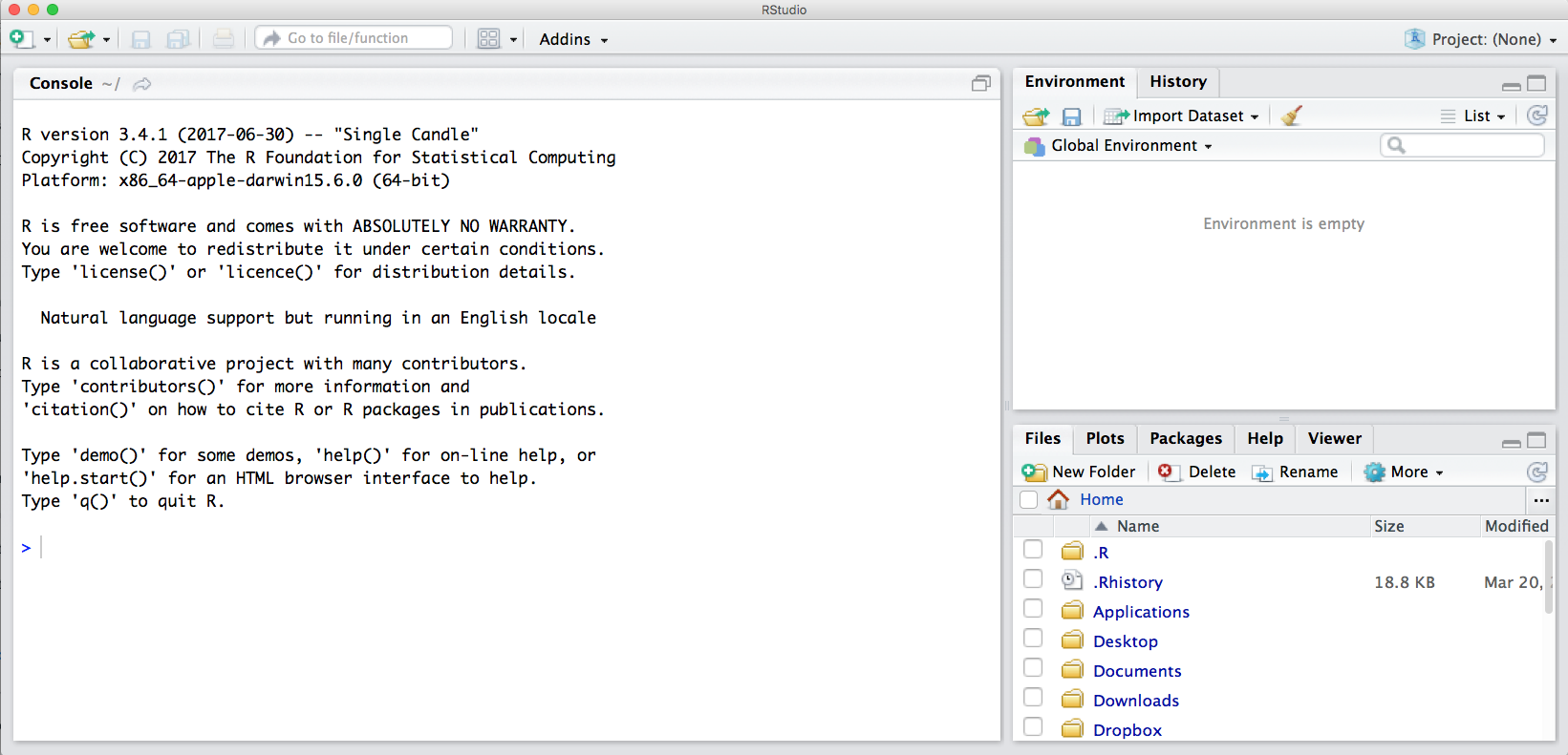
The default RStudio setup has a few panes that you will use. Here they are with their default locations:

Console (entire left)
Environment/History (tabbed in upper right)
Files/Plots/Packages/Help (tabbed in lower right)

You can change the default location of the panes, among many other things: Customizing RStudio.

One key question to ask whenever we open up RStudio is “where am I?” Because we like to work in RStudio projects, often this question is synonymous with “what project am I in?” In our setup we have already worked with R projects a little, but haven’t explained much about what they are or why we use them.

An R project is really a special kind of working directory, which has its own workspace, history, and settings. Even though it isn’t much more than a special folder, it is a powerful way to organize your work.

There are two places that can indicate what project we are in. The first is the project switcher menu in the upper right hand corner of your RStudio window. The second is the working directory path, in the top bar of your console. Note that by default, your working directory is set to the top level of your R project directory unless you change it using the setwd() function.

Setting up git

Before using git, you need to tell it who you are, also known as setting the global options. The only way to do this is through the command line. Newer versions of RStudio have a nice feature where you can open a terminal window in your RStudio session. Do this by selecting Tools -> Terminal -> New Terminal.

A terminal tab should now be open where your console usually is.

To set the global options, type the following into the command prompt, with your actual name, and press enter:

git config --global user.name "Halina Do-Linh"

Note that if it runs successfully, it will look like nothing happened. We will check at the end to make sure it worked.

Next, enter the following line, with the email address you used when you created your account on github.com:

git config --global user.email "username@github.com"

Note that these lines need to be run one at a time.

Next, we will set our credentials to not time out for a very long time. This is related to the way that our server operating system handles credentials - not doing this will make your PAT (which we will set up soon) expire immediately on the system, even though it is actually valid for a month.

git config --global credential.helper 'cache --timeout=10000000'

Finally, check to make sure everything looks correct by entering this command, which will return the options that you have set.

git config --global --list

1.2.7.2 GitHub Authentication

GitHub recently deprecated password authentication for accessing repositories, so we need to set up a secure way to authenticate. The book Happy git with R has a wealth of information related to working with git in R, and these instructions are based off of section 10.1.

We will be using a PAT (Personal Access Token) in this course, because it is easy to set up. For better security and long term use, we recommend taking the extra steps to set up SSH keys.

Steps:

Run usethis::create_github_token() in the console
In the browser window that pops up, scroll to the bottom and click “generate token.” You may need to log into GitHub first.
Copy the token from the green box on the next page
Back in RStudio, run credentials::set_github_pat()
Paste your token into the dialog box that pops up.

1.2.8 Setting up the R environment on your local computer

R Version

We will use R version 4.0.5, which you can download and install from CRAN. To check your version, run this in your RStudio console:

R.version$version.string

If you have R version 4.0.0 that will likely work fine as well.

RStudio Version

We will be using RStudio version 1.4 or later, which you can download and install here To check your RStudio version, run the following in your RStudio console:

RStudio.Version()$version

If the output of this does not say 1.4 or higher, you should update your RStudio. Do this by selecting Help -> Check for Updates and follow the prompts.

Package installation

Run the following lines to check that all of the packages we need for the training are installed on your computer.

packages <- c("dplyr", "tidyr", "readr", "devtools", "usethis", "roxygen2", "leaflet", "ggplot2", "DT", "scales", "shiny", "sf", "ggmap", "broom", "captioner", "MASS")

for (package in packages) {
    
    if (!(package %in% installed.packages())) { install.packages(package) }
    
    }

rm(packages) # remove variable from workspace

# Now upgrade any out-of-date packages
update.packages(ask=FALSE)

If you haven’t installed all of the packages, this will automatically start installing them. If they are installed, it won’t do anything.

Next, create a new R Markdown (File -> New File -> R Markdown). If you have never made an R Markdown document before, a dialog box will pop up asking if you wish to install the required packages. Click yes.

At this point, RStudio and R should be all set up.

Setting up git locally

If you haven’t downloaded git already, you can do so here.

If you haven’t already, go to github.com and create an account.

Then you can follow the instructions that we used above to set your email address and user name.

Note for Windows Users

If you get “command not found” (or similar) when you try these steps through the RStudio terminal tab, you may need to set the type of terminal that gets launched by RStudio. Under some git install scenarios, the git executable may not be available to the default terminal type. Follow the instructions on the RStudio site for Windows specific terminal options. In particular, you should choose “New Terminals open with Git Bash” in the Terminal options (Tools->Global Options->Terminal).

In addition, some versions of windows have difficulty with the command line if you are using an account name with spaces in it (such as “Matt Jones,” rather than something like “mbjones”). You may need to use an account name without spaces.

Updating a previous R installation

This is useful for users who already have R with some packages installed and need to upgrade R, but don’t want to lose packages. If you have never installed R or any R packages before, you can skip this section.

If you already have R installed, but need to update, and don’t want to lose your packages, these two R functions can help you. The first will save all of your packages to a file. The second loads the packages from the file and installs packages that are missing.

Save this script to a file (e.g. package_update.R).

#' Save R packages to a file. Useful when updating R version
#'
#' @param path path to rda file to save packages to. eg: installed_old.rda
save_packages <- function(path){
    
    tmp <- installed.packages()
    installedpkgs <- as.vector(tmp[is.na(tmp[,"Priority"]), 1])
    save(installedpkgs, file = path)
}

#' Update packages from a file. Useful when updating R version
#' 
#' @param path path to rda file where packages were saved
update_packages <- function(path){
    tmp <- new.env()
    installedpkgs <- load(file = path, envir = tmp)
    installedpkgs <- tmp[[ls(tmp)[1]]]
    tmp <- installed.packages()

    installedpkgs.new <- as.vector(tmp[is.na(tmp[,"Priority"]), 1])
    missing <- setdiff(installedpkgs, installedpkgs.new)
    install.packages(missing)
    update.packages(ask=FALSE)
}

Source the file that you saved above (eg: source(package_update.R)). Then, run the save_packages function.

save_packages("installed.rda")

Then quit R, go to CRAN, and install the latest version of R.

Source the R script that you saved above again (eg: source(package_update.R)), and then run:

update_packages("installed.rda")

This should install all of your R packages that you had before you upgraded.