14  Zarr for Cloud Data Storage

14.1 Learning Objectives

• Understand the principles of the Zarr file format
• Recognize the primary use case for Zarr
• Learn to access an example Zarr dataset from Google Cloud Storage

14.2 Introduction

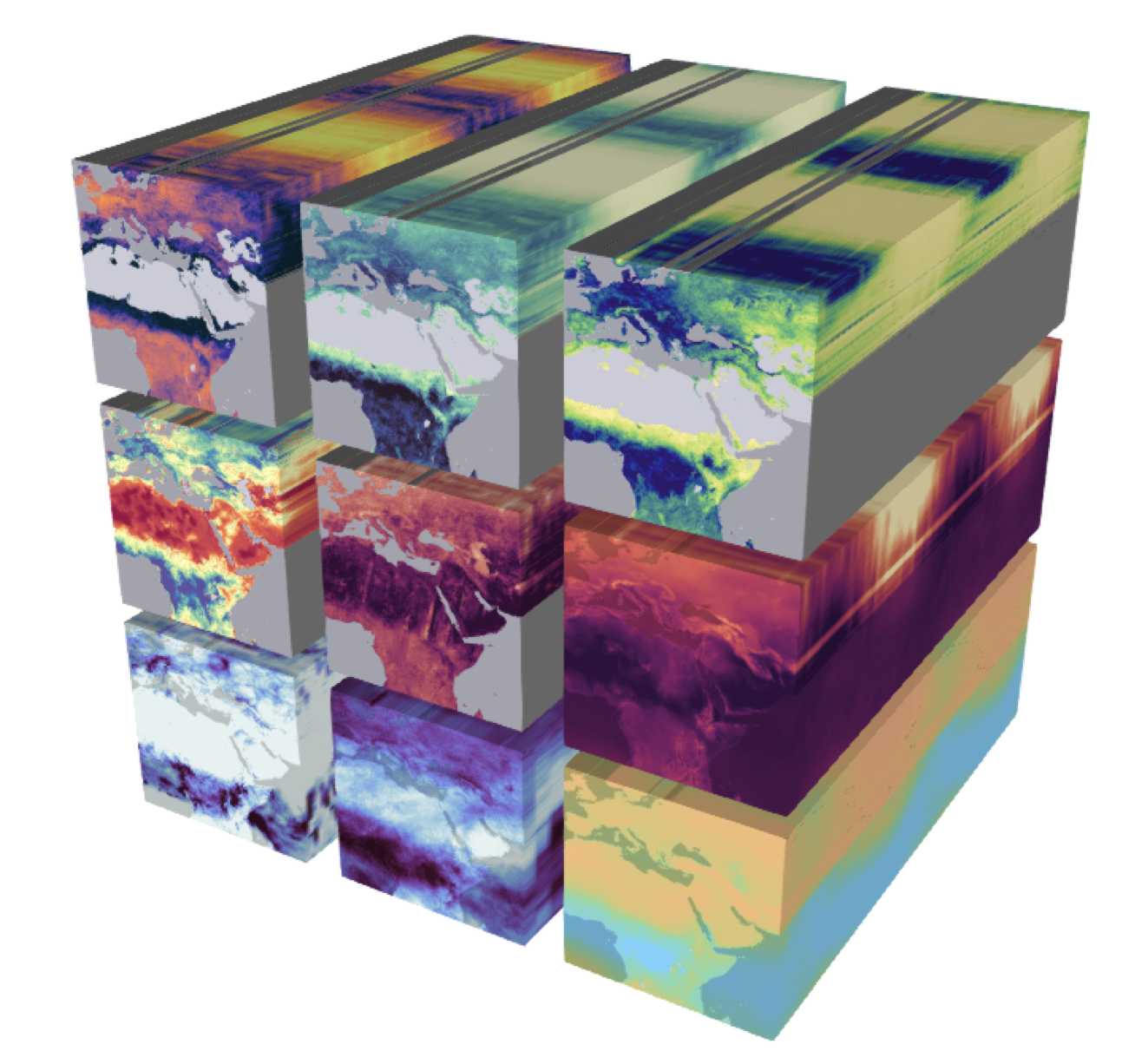
In working with Earth systems data, it is common to have datasets that have multiple dimensions. Remember from the lesson on data structures for large data the diagram below, showing an Earth system data cube with 9 variables and 3 measurement dimensions. When we work with data like this, we need to make sure that we store it in a format that allows us to store the data efficiently, access it easily, and understand it correctly. The NetCDF format achieves all of these goals, and is widely used for multi-dimensional datasets. The NetCDF format does have some limitations though, and the increasing use of distributed computing in Earth science research makes the utility of a cloud-optimized NetCDF-like format clear.

Mahecha et al. 2020 . Visualization of the implemented Earth system data cube. The figure shows from the top left to bottom right the variables sensible heat (H), latent heat (LE), gross primary production (GPP), surface moisture (SM), land surface temperature (LST), air temperature (Tair), cloudiness (C), precipitation (P), and water vapour (V). The resolution in space is 0.25° and 8 d in time, and we are inspecting the time from May 2008 to May 2010; the spatial range is from 15° S to 60° N, and 10° E to 65° W.

Cloud computing is distributed - meaning that files and processes are spread around different pieces of hardware that may or may not be located in the same place. There is great power in this - it enables flexibility and scalability of systems - but there are challenges associated with it too. One of those challenges is data storage and access. Medium sized datasets, like we have seen so far, work great in a NetCDF file accessed by tools like xarray. What happens though, when datasets get extremely large, in the range of multiple terabytes or even petabytes. Storing a couple of TB of data in a single netCDF file is not practical in most cases - especially when you are trying to leverage distributed computing, where there are multiple places where files are stored. Of course, one could (and many have) artificially split that terabyte scale dataset into multiple files, such as daily observations. This is fine - but what if even the daily data is too large for a single file? What if the total volume of files is too large for one hard drive? How would you keep track of what file is where? The Zarr file format is meant to solve these problems and more, making it easier to access data on distributed systems.

“Zarr is a file storage format for chunked, compressed, N-dimensional arrays based on an open-source specification.” If this sounds familiar - it should! Zarr shares many characteristics in terms of functionality and design with NetCDF. Below is a mapping of NetCDF and Zarr terms from the NASA earthdata wiki

NetCDF Model	Zarr Model
File	Store
Group	Group
Variable	Array
Attribute	User Attribute
Dimension	(Not supported natively)

The first thing to notice about this list is that the terms are very similar. NetCDF and Zarr share many characteristics, and when working with the data from those file types in python, the workflows are nearly identical. The first of the above listed terms, however, highlights the biggest difference between NetCDF and Zarr. While NetCDF is a file, the Zarr model instead is a “store.” Rather than storing all of the data in one file, Zarr stores data in a directory where each file is a chunk of data. Below is a diagram, also from the earthdata wiki, showing an example layout.

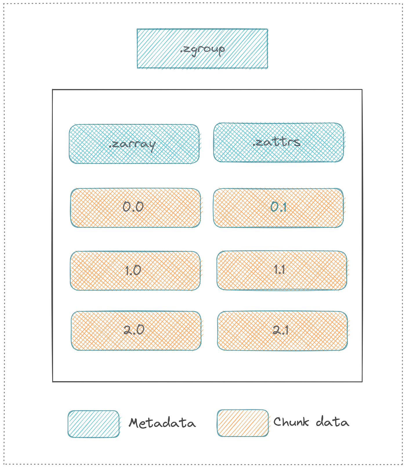
In this layout diagram, key elements of the Zarr specification are introduced.

• Array: a multi-dimensional, chunked dataset
• Attribute: ancillary data or metadata in key-value pairs
• Group: a container for organizing multiple arrays or sub-groups within a hierarchical structure
• Metadata: key information enabling correct interpretation of stored data format, eg shape, chunk dimensions, compression, and fill value.

The chunked arrays and groups allow for easier distributed computing, and enable a high degree of parallelism. Because the chunks are in seperate files, you can run concurrent operations on different parts of the same dataset, and the dataset itself can exist on multiple nodes in a cluster or cloud computing configuration. Because Zarr is laid out as a store and not a series of self contained files (like NetCDF), it means the entire dataset can be accessed via a single remote URI. This not only can make analysis more streamlined, but it also means that you don’t have to store any part of the dataset locally. The Zarr format, when used with xarray, also allows for working with datasets too large to fit into local memory. A high degree of flexibility in compression and filtering schemes also means that chunks can be stored extremely efficiently.

14.3 Using Zarr

Zarr is a file format, which has implementations in several languages. The primary implementation is in Python, but there is also support in Java and R. Here, we will look at an example of how to use the Zarr format by looking at some features of the zarr library and how Zarr files can be opened with xarray.

14.4 Retrieving CMIP6 Data from Google Cloud

Here, we will show how to uze Zarr and xarray to read in the CMIP6 climate model data from the World Climate Research Program, hosted by Googe Cloud. CMIP6 is a huge set of climate models, with around 100 models produced across 49 different groups. There is an enormous amount of data produced by these models, and in this demonstration we will load a tiny fraction of it. This demonstration is based off of an example put together by Pangeo

First we’ll load some libraries. pandas, numpy, and xarray should all be familiar by now. We’ll also load in zarr, of course, and gcsfs, the Google Cloud Storage File System library, which enables access to Google Cloud datasets, including our CMIP6 example.

import pandas as pd
import numpy as np
import zarr
import xarray as xr
import gcsfs

Next, we’ll read a csv file that contains information about all of the CMIP6 stores available on Google Cloud. You can find this URL to this csv file by navigating to the Google Cloud CMIP6 home page, clicking on “View Dataset,” and pressing the copy link button for the file in the table.

df = pd.read_csv('https://storage.googleapis.com/cmip6/cmip6-zarr-consolidated-stores.csv')
df.head()

	activity_id	institution_id	source_id	experiment_id	member_id	table_id	variable_id	grid_label	zstore	dcpp_init_year	version
0	HighResMIP	CMCC	CMCC-CM2-HR4	highresSST-present	r1i1p1f1	Amon	ps	gn	gs://cmip6/CMIP6/HighResMIP/CMCC/CMCC-CM2-HR4/...	NaN	20170706
1	HighResMIP	CMCC	CMCC-CM2-HR4	highresSST-present	r1i1p1f1	Amon	rsds	gn	gs://cmip6/CMIP6/HighResMIP/CMCC/CMCC-CM2-HR4/...	NaN	20170706
2	HighResMIP	CMCC	CMCC-CM2-HR4	highresSST-present	r1i1p1f1	Amon	rlus	gn	gs://cmip6/CMIP6/HighResMIP/CMCC/CMCC-CM2-HR4/...	NaN	20170706
3	HighResMIP	CMCC	CMCC-CM2-HR4	highresSST-present	r1i1p1f1	Amon	rlds	gn	gs://cmip6/CMIP6/HighResMIP/CMCC/CMCC-CM2-HR4/...	NaN	20170706
4	HighResMIP	CMCC	CMCC-CM2-HR4	highresSST-present	r1i1p1f1	Amon	psl	gn	gs://cmip6/CMIP6/HighResMIP/CMCC/CMCC-CM2-HR4/...	NaN	20170706

CMIP6 is an extremely large collection of datasets, with their own terminology. We’ll be making a request based on the experiment id (scenario), table id (tables are organized roughly by themes), and variable id.

For this example, we’ll select data from a simulation of the recent past (historical) from the ocean daily (Oday) table, and select the sea surface height (tos) variable. We’ll also only select results from NOAA Geophysical Fluid Dynamics Laboratory (NOAA-GFDL) runs. We’ll do this by passing a logical statment with these criteria to the query method of our pandas data.frame.

df_ta = df.query("activity_id=='CMIP' & table_id == 'Oday' & variable_id == 'tos' & experiment_id == 'historical' & institution_id == 'NOAA-GFDL'")
df_ta

	activity_id	institution_id	source_id	experiment_id	member_id	table_id	variable_id	grid_label	zstore	dcpp_init_year	version
9445	CMIP	NOAA-GFDL	GFDL-CM4	historical	r1i1p1f1	Oday	tos	gr	gs://cmip6/CMIP6/CMIP/NOAA-GFDL/GFDL-CM4/histo...	NaN	20180701
9446	CMIP	NOAA-GFDL	GFDL-CM4	historical	r1i1p1f1	Oday	tos	gn	gs://cmip6/CMIP6/CMIP/NOAA-GFDL/GFDL-CM4/histo...	NaN	20180701
244828	CMIP	NOAA-GFDL	GFDL-ESM4	historical	r1i1p1f1	Oday	tos	gn	gs://cmip6/CMIP6/CMIP/NOAA-GFDL/GFDL-ESM4/hist...	NaN	20190726
244829	CMIP	NOAA-GFDL	GFDL-ESM4	historical	r1i1p1f1	Oday	tos	gr	gs://cmip6/CMIP6/CMIP/NOAA-GFDL/GFDL-ESM4/hist...	NaN	20190726

Note in the table above there is a column zstore. This gives the URI for the store described in each row of the dataset. Note there is also a version column indicating the date of that particular version. We will use both of these columns to select a single store of data.

First, though, we need to set up a connection to the Google Cloud Storage file system (GCSFS). We do this using the gcsfs library to call the GCSFileSystem method using an anonymous token. Because this dataset is completely open, we do not have to authenticate at all to access it.

gcs = gcsfs.GCSFileSystem(token='anon')

Now, we’ll create a variable with the path to the most recent store from the table above (note the table is sorted by version, so we grab the store URL from the last row), and create a mapping interface to the store using the connection to the Google Cloud Storage system. This interface is what allows us to access the Zarr store with all of the data we are interested in.

zstore = df_ta.zstore.values[-1]
mapper = gcs.get_mapper(zstore)

Nex, we open the store using the xarray method open_zarr and examine its metadata. Note that the first argument to open_zarr can be a “MutableMapping where a Zarr Group has been stored” (what we are using here), or a path to a directory in file system (if a local Zarr store is being used).

ds = xr.open_zarr(mapper)
ds

This piece of data is around 30 GB total, and we made it accessible to our environment nearly instantly. Consider also that the total volume of CMIP6 data available on Google Cloud is in the neighborhood of a few petabytes, and it is all available at your fingertips using Zarr.

From here, using the xarray indexing, we can easily grab a time slice and make a plot of the data.

ds.tos.sel(time='1999-01-01').squeeze().plot()

We can also get a timeseries slice, here on the equator in the Eastern Pacific.

ts = ds.tos.sel(lat = 0, lon = 272, method = "nearest")

xarray allows us to do some pretty cool things, like calculate a rolling annual mean on our daily data. Again, because none of the data are loaded into memory, it is nearly instant.

ts_ann = ts.rolling(time = 365).mean()

Note that if we explicitly want to load the data into memory, we can by using the load method.

ts.load()

ts_ann.load()

Finally, we can make a simple plot of the daily temperatures, along with the rolling annual mean.

ts.plot(label = "daily")
ts_ann.plot(label = "rolling annual mean")

As an additional example, let’s look at some ocean nitrate and phosphorous data. These tasks take a little longer since the data have an additional dimension - ocean depth.

First, let’s get the nitrate data by looking at the no3 variable.

no3 = df.query("activity_id=='CMIP' & table_id == 'Omon' & experiment_id == 'historical' & institution_id == 'NOAA-GFDL' & variable_id == 'no3'")
ds_no3 = xr.open_zarr(gcs.get_mapper(no3.zstore.values[-1]), consolidated=True)

We’ll also get the po4 variable.

po4 = df.query("activity_id=='CMIP' & table_id == 'Omon' & experiment_id == 'historical' & institution_id == 'NOAA-GFDL' & variable_id == 'po4'")
ds_po4 = xr.open_zarr(gcs.get_mapper(po4.zstore.values[-1]), consolidated=True)

Now, use xarray methods to select data from the 2.5 level, and calculate the mean over time.

Answer

no3_mean = ds_no3.no3.sel(lev = 2.5).mean('time').squeeze().load()po4_mean = ds_po4.po4.sel(lev = 2.5).mean('time').squeeze().load()

import matplotlib.pyplot as plt
plt.scatter(z_mean, t_mean)

In this simple demonstration we used less than 20 lines of code to establish access to a multi-petabyte climate dataset, extract a relevant variable, calculate a rolling average, and make two plots. The advent of cloud computing and cloud-native formats like Zarr are completely changing how we can do science. In their abstract for a talk on the process of storing these data on Google Cloud, Henderson and Abernathy (2020) give the motivation:

Aha! You have an awe-inspiring insight and can’t wait to share your results. Then an advisor/colleague/reviewer asks “But what do the CMIPx models say?”. In 2008, with the 35Tb of CMIP3 data, you could, perhaps, come up with an answer in a few days, collecting needed data for all available models, making the time and space uniform, checking units and running your analysis. (Henderson and Abernathey 2020)

A few days seems optimistic, even, for sifting through 35TB of data. Imagine the process of finding, manually downloading, harmonizing, etc. many petabytes of CMIP6 data. The availability of these commonly used datasets via seamless tooling with the Pangeo universe of packages, has, to paraphrase the above abstract, has the potential to seriously accelerate earth and environmental science research.

14.5 Additional Reference: Creating a Zarr Dataset

This is a simplified version of the official Zarr tutorial.

First, create an array of 10,000 rows and 10,000 columns, filled with zeros, divided into chunks where each chunk is 1,000 x 1,000.

import zarr
import numpy as np
z = zarr.zeros((10000, 10000), chunks=(1000, 1000), dtype='i4')
z

<zarr.core.Array (10000, 10000) int32>

The array can be treated just like a numpy array, where you can assign values using indexing.

z[0, :] = np.arange(10000)
z[:]

array([[   0,    1,    2, ..., 9997, 9998, 9999],
       [   0,    0,    0, ...,    0,    0,    0],
       [   0,    0,    0, ...,    0,    0,    0],
       ...,
       [   0,    0,    0, ...,    0,    0,    0],
       [   0,    0,    0, ...,    0,    0,    0],
       [   0,    0,    0, ...,    0,    0,    0]], dtype=int32)

To save the file, just use the save method.

zarr.save('data/example.zarr', z)

And open to open it again.

arr = zarr.open('data/example.zarr')
arr

<zarr.core.Array (10000, 10000) int32>

To create groups in your store, use the create_group method after creating a root group. Here, we’ll create two groups, temp and precip.

root = zarr.group()
temp = root.create_group('temp')
precip = root.create_group('precip')

You can then create a dataset (array) within the group, again specifying the shape and chunks.

t100 = temp.create_dataset('t100', shape=(10000, 10000), chunks=(1000, 1000), dtype='i4')
t100

<zarr.core.Array '/temp/t100' (10000, 10000) int32>

Groups can easily be accessed by name and index.

root['temp']
root['temp/t100'][:, 3]

array([0, 0, 0, ..., 0, 0, 0], dtype=int32)

To get a look at your overall dataset, the tree and info methods are helpful.

root.tree()

root.info

Name	/
Type	zarr.hierarchy.Group
Read-only	False
Store type	zarr.storage.MemoryStore
No. members	2
No. arrays	0
No. groups	2
Groups	precip, temp

Henderson, N., and R. Abernathey. 2020. “CMIP6 in the Cloud - Why?”