install.packages("skimr")13.1 Data Quality
Learning objectives:
- How the Arctic Data Center evaluates data quality
- How to use R to evaluate data quality
13.1.1 Automated Data Quality Assessment at the Arctic Data Center
The Arctic Data Center performs automated metadata and data quality assessments of every dataset shortly after it is submitted. Each assessment consists of a series of checks that are performed on either the metadata or data (or both!) contained within the dataset. Within what is called a “suite” of checks, the checks are classified into either required, optional, or informational checks. Additionally, they are classified into FAIR categories, where FAIR represents Findable, Accessible, Interoperable, Reusable.
An overall score is then calculated for each dataset, according to the following formula:
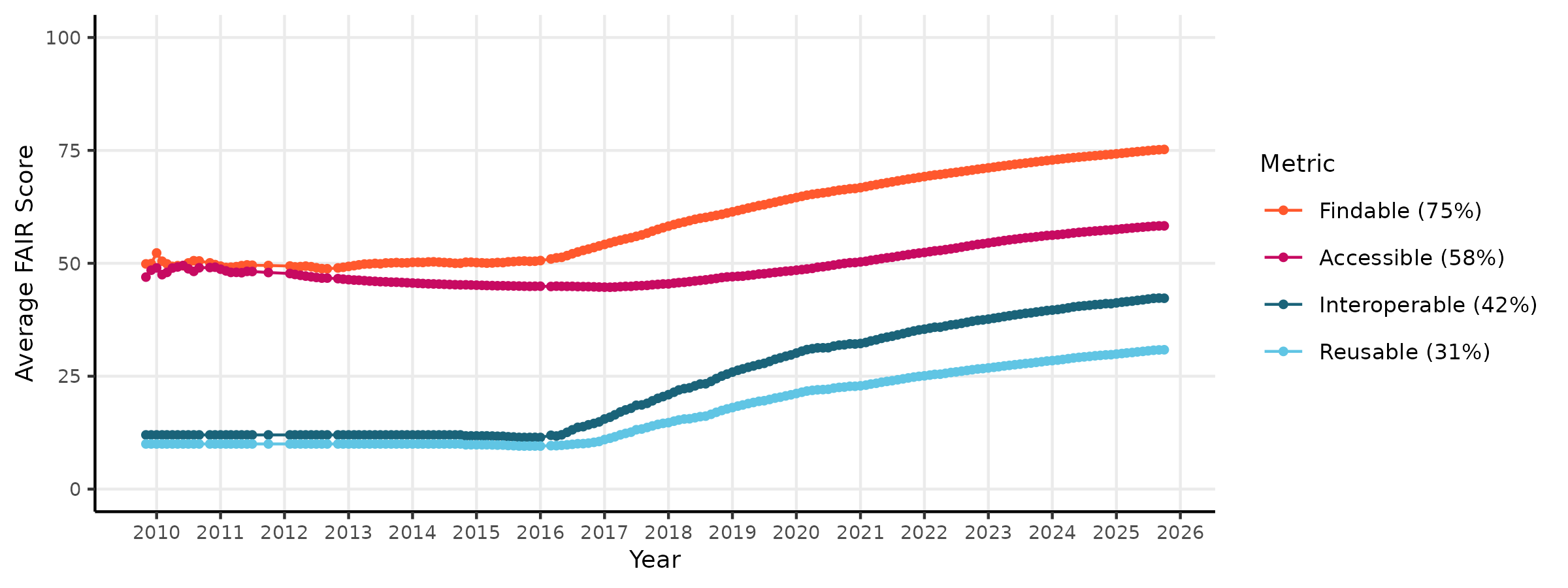
\[score = \frac{R_{pass} + O_{pass}}{R_{pass} + R_{fail} + O_{pass}}\] where R is the number of Required checks that pass or fail, and O is the number of Optional checks that pass or fail. This ensures that datasets are not penalized for failing optional checks. This system allows the Arctic Data Center to evaluate FAIR-ness of its datasets over time. The figure below shows the quality scores of the repository through time for metadata FAIRness.
 To evaluate data quality over a wide range of data types and disciplines, the Arctic Data Center first conceptualized four categories of data quality checks. These categories are: congruency, accessibility, validity, and accuracy.
Congruency
Is the file what it says it is?
- data format matches format listed
- checksum of file matches documentation
- variable names in file match documentation
Accessibility
Can the file be accessed and read correctly?
- text formatted files valid according to subtype (eg: csv files match format)
- binary files validate against declared type (eg: hdf5 is valid against HDF5 standard)
- characters in text files are valid against declared encoding
Validity
Are values valid within reasonable bounds?
- air temperatures within -100 and 100 degrees C
- ocean depth does not exceed 10,935m
- tree diameters do not get smaller through time
Accuracy
Does this value make sense given the other values?
- statistical outliers in measured variables
- anomalous NDVI values caused by cloud interference
At the Arctic Data Center, we have chosen to tackle the first two types of data checks, since they are domain agnostic and do not require specialized knowledge to implement the checks. So far, the data suite we have developed has implemented the following checks:
| Check ID | Description |
|---|---|
| All files | Content malware-free |
| All files | Data format congruent with metadata |
| All files | Data content not zipped unless it is a shapefile set |
| Text files | Text encoding valid according to guessed format |
| Text delimited tables | Table variables congruent with metadata |
| Text delimited tables | Table well-formed |
| Text delimited tables | Column names printable |
| Text delimited tables | Columns and rows contain data |
| Text delimited tables | Dates parse correctly according to metadata |
| Text delimited tables | Latitude/longitude data congruent with metadata |
| Text delimited tables | Missing values documented |
| Text delimited tables | Shows a glimpse of a table |
| Shapefiles | Shapefile sets complete |
| Shapefiles | Shapefile coordinates within CRS bounds |
| Shapefiles | Shapefile geometry congruent with metadata |
| NetCDF files | NetCDF global attributes complete |
| NetCDF files | NetCDF variable attributes complete |
| NetCDF files | NetCDF coordinate attributes complete |
| Raster files | Raster well-formed |
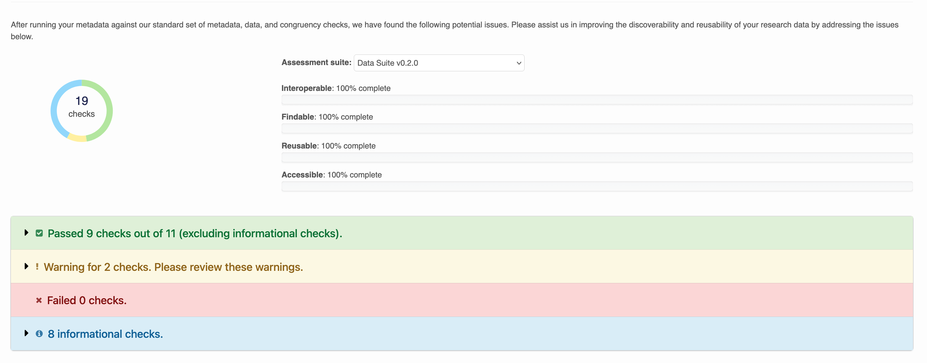
When these checks are run, each dataset recieves a report like the below:
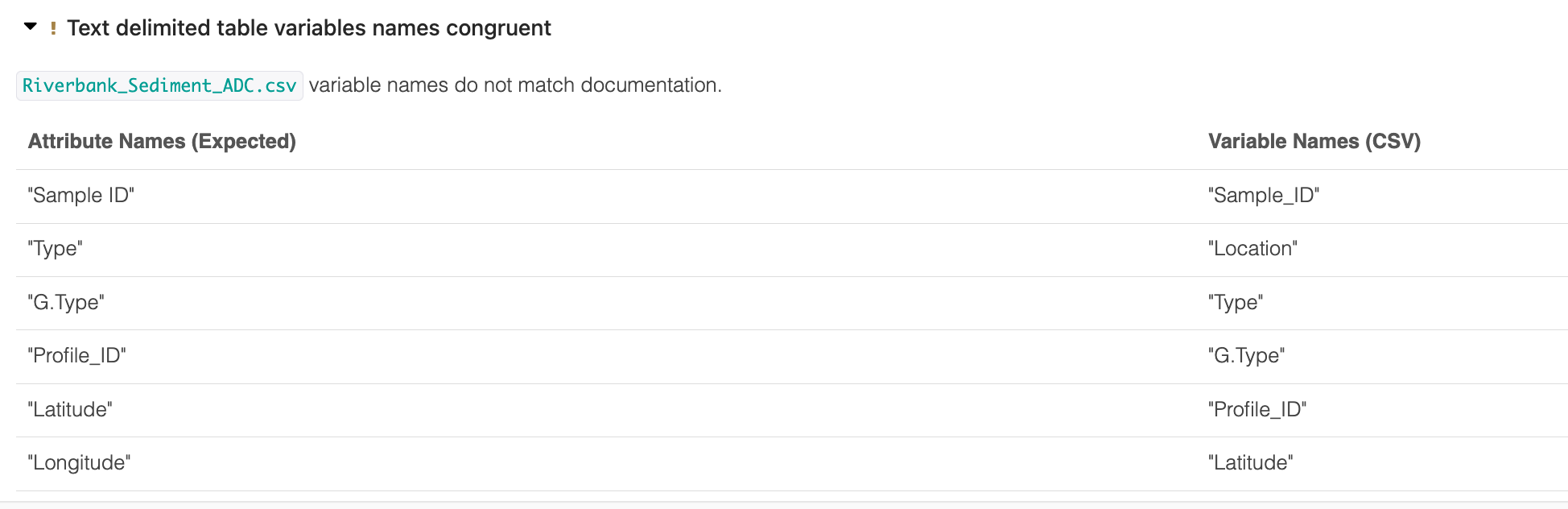
Warnings are issued for checks that failed, but are optional. Within each row, output describes the result of the check. For example: Column names in Riverbank_Sediment_ADC.csv are well formed. No non-printable characters detected.
Some output is collapsed for readability:
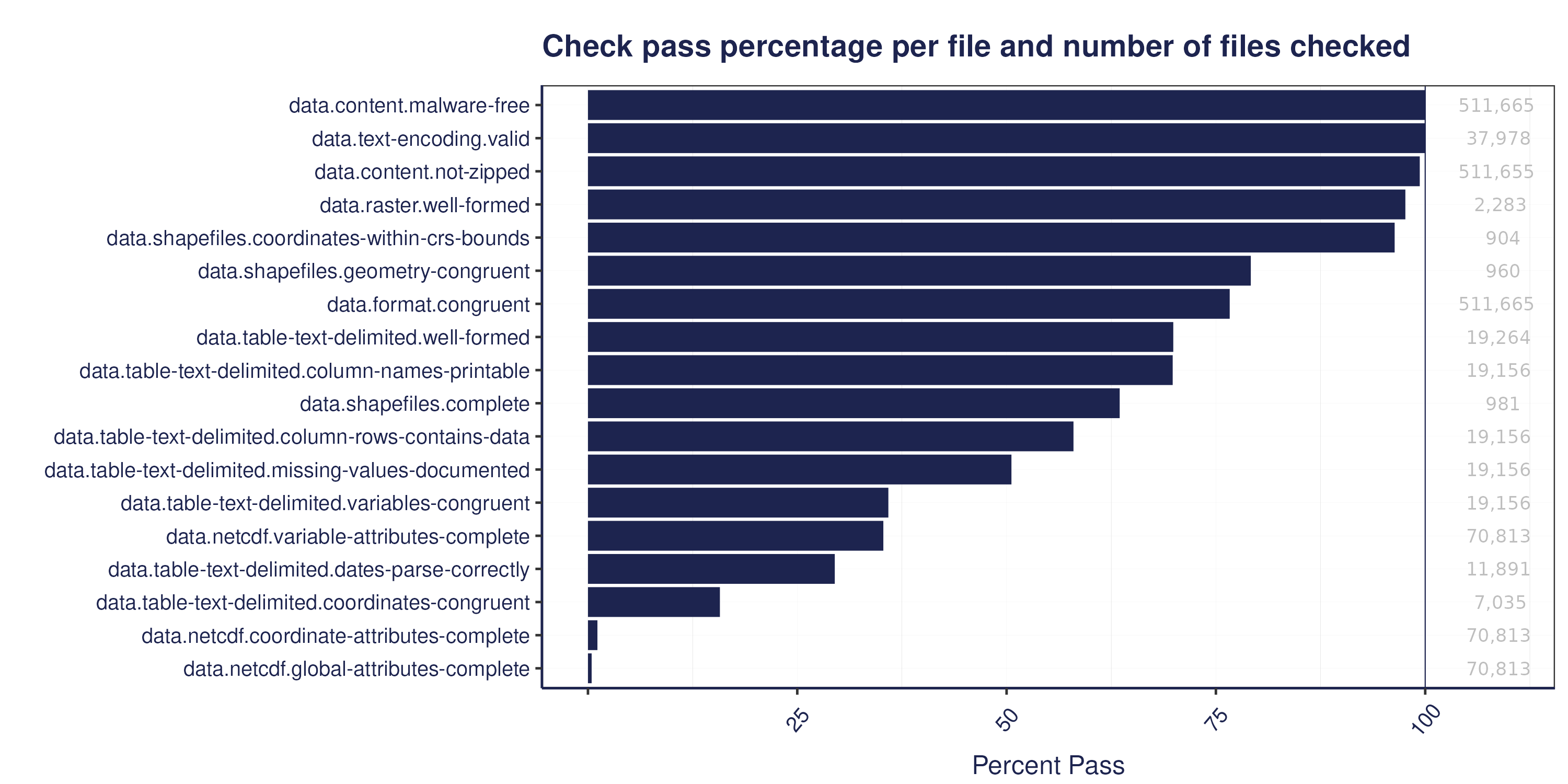
 The figure below shows a summary of the percentage of files that pass our data quality checks, by check:
13.1.2 Checking Data Quality in R
Poll:
- What are the most common quality issues you see?
- What kind of data quality checks do you use on your own data?
- Do you have ideas for checks you think we should add to the ADC quality suite?
Although the Arctic Data Center has implemented data quality checks that are automated, the vast majority of data quality work still falls on researchers doing analysis. In this section we will discuss a few tools that researchers can use in R to do general data quality work.
13.1.2.1 Resolving mysteries with file
When a researcher receives a new file to incorporate into an analysis, the first step is to examine the file. One tool already used in the Arctic Data Center data quality suite is the file utility in linux/unix systems. This is a command run using the terminal that performs tests on the content of a file to determine its type. This is useful for files where the type is unknown, or for files that cannot be read into R for unknown reasons.
In the terminal, run the following:
file data/BGchem2008data.csvYou should see an output like: data/BGchem2008data.csv: CSV text. Which makes sense!
The file command is very helpful at catching things like this, where we have an excel file masquerading as a csv file. You might wind up using this if you try to read in the example file below using read.csv, and get output that looks completely garbled.
file example-data/my-data.csv
example-data/my-data.csv: Microsoft Excel 2007+
Another great use of the file command is for mystery extensions:
file example-data/JUSTIN_400__001.DZG
example-data/JUSTIN_400__001.DZG: ASCII text, with CRLF, LF line terminators
13.1.2.2 Quick Summaries with skimr and visdat
First, we need to install the skimr package.
And load it into our environment, along with readr
library(skimr)
library(readr)
library(dplyr)
library(lubridate)
Now we’ll read in a familar file, the BGChem2008data.csv from Craig Tweedie. (2009). North Pole Environmental Observatory Bottle Chemistry. Arctic Data Center. doi:10.18739/A25T3FZ8X.
bg_chem <- read_csv("data/BGchem2008data.csv")Rows: 70 Columns: 19
── Column specification ────────────────────────────────────────────────────────
Delimiter: ","
chr (1): Station
dbl (16): Latitude, Longitude, Target_Depth, CTD_Depth, CTD_Salinity, CTD_T...
dttm (1): Time
date (1): Date
ℹ Use `spec()` to retrieve the full column specification for this data.
ℹ Specify the column types or set `show_col_types = FALSE` to quiet this message.Notice that the read_csv call already gives us some information about the dataset here. It tells us what the columns are, and what the column types are. skimr can give us even more information that will be helpful.
skim(bg_chem)| Name | bg_chem |
| Number of rows | 70 |
| Number of columns | 19 |
| _______________________ | |
| Column type frequency: | |
| character | 1 |
| Date | 1 |
| numeric | 16 |
| POSIXct | 1 |
| ________________________ | |
| Group variables | None |
Variable type: character
| skim_variable | n_missing | complete_rate | min | max | empty | n_unique | whitespace |
|---|---|---|---|---|---|---|---|
| Station | 0 | 1 | 8 | 11 | 0 | 15 | 0 |
Variable type: Date
| skim_variable | n_missing | complete_rate | min | max | median | n_unique |
|---|---|---|---|---|---|---|
| Date | 0 | 1 | 2008-03-21 | 2008-03-30 | 2008-03-26 | 9 |
Variable type: numeric
| skim_variable | n_missing | complete_rate | mean | sd | p0 | p25 | p50 | p75 | p100 | hist |
|---|---|---|---|---|---|---|---|---|---|---|
| Latitude | 0 | 1 | 74.04 | 1.37 | 72.05 | 72.97 | 74.05 | 75.26 | 76.32 | ▇▇▆▇▆ |
| Longitude | 0 | 1 | -148.11 | 7.98 | -163.70 | -153.27 | -149.81 | -140.31 | -136.54 | ▃▃▇▅▇ |
| Target_Depth | 0 | 1 | 123.79 | 106.04 | 20.00 | 60.00 | 85.00 | 190.00 | 430.00 | ▇▁▂▂▁ |
| CTD_Depth | 0 | 1 | 125.42 | 107.70 | 15.13 | 60.34 | 85.78 | 192.66 | 442.17 | ▇▁▂▂▁ |
| CTD_Salinity | 0 | 1 | 31.45 | 2.31 | 25.50 | 30.17 | 31.65 | 33.08 | 34.82 | ▂▂▆▇▇ |
| CTD_Temperature | 0 | 1 | -0.96 | 0.66 | -1.68 | -1.49 | -1.26 | -0.48 | 0.70 | ▇▂▂▁▂ |
| Bottle_Salinity | 0 | 1 | 31.45 | 2.31 | 25.50 | 30.17 | 31.65 | 33.08 | 34.82 | ▂▂▆▇▇ |
| d18O | 0 | 1 | -2.02 | 1.12 | -3.73 | -2.96 | -2.04 | -1.49 | 0.21 | ▆▃▇▁▃ |
| Ba | 0 | 1 | 60.95 | 35.20 | -99.00 | 64.08 | 69.68 | 72.25 | 86.09 | ▁▁▁▁▇ |
| Si | 0 | 1 | 13.29 | 11.32 | 2.46 | 3.92 | 8.42 | 20.98 | 36.58 | ▇▃▁▁▂ |
| NO3 | 0 | 1 | 6.86 | 6.12 | -0.05 | 0.78 | 4.75 | 13.04 | 15.85 | ▇▂▁▂▅ |
| NO2 | 0 | 1 | 0.05 | 0.06 | 0.00 | 0.01 | 0.02 | 0.04 | 0.27 | ▇▁▁▁▁ |
| NH4 | 0 | 1 | 0.06 | 0.07 | 0.01 | 0.02 | 0.03 | 0.07 | 0.37 | ▇▁▁▁▁ |
| P | 0 | 1 | 1.12 | 0.42 | 0.57 | 0.80 | 0.97 | 1.50 | 1.87 | ▇▇▂▁▅ |
| TA | 0 | 1 | 2089.08 | 478.16 | -99.00 | 2135.50 | 2203.10 | 2270.99 | 2312.30 | ▁▁▁▁▇ |
| O2 | 0 | 1 | -73.06 | 46.14 | -99.00 | -99.00 | -99.00 | -99.00 | 9.25 | ▇▁▁▁▂ |
Variable type: POSIXct
| skim_variable | n_missing | complete_rate | min | max | median | n_unique |
|---|---|---|---|---|---|---|
| Time | 0 | 1 | 1899-12-31 00:19:50 | 1899-12-31 23:50:29 | 1899-12-31 20:52:24 | 15 |
skim gives us information about the data frame including basic statistics on the numeric values, missing values, and number of unique values in the character variables.
Helpfully, skim can also handle grouped output, if we wanted to look more closely at summaries of oxygen concentaration by station, for example, we can run:
bg_chem %>%
  select(Station, O2) %>%
  group_by(Station) %>%
skim()| Name | Piped data |
| Number of rows | 70 |
| Number of columns | 2 |
| _______________________ | |
| Column type frequency: | |
| numeric | 1 |
| ________________________ | |
| Group variables | Station |
Variable type: numeric
| skim_variable | Station | n_missing | complete_rate | mean | sd | p0 | p25 | p50 | p75 | p100 | hist |
|---|---|---|---|---|---|---|---|---|---|---|---|
| O2 | 72N,140W | 0 | 1 | -27.59 | 55.32 | -99 | -72.64 | 7.18 | 8.65 | 9.19 | ▃▁▁▁▇ |
| O2 | 72N,150W | 0 | 1 | -99.00 | 0.00 | -99 | -99.00 | -99.00 | -99.00 | -99.00 | ▁▁▇▁▁ |
| O2 | 72_40N,145W | 0 | 1 | -56.25 | 58.55 | -99 | -99.00 | -99.00 | 6.54 | 9.23 | ▇▁▁▁▅ |
| O2 | 73N,140W | 0 | 1 | -56.22 | 58.59 | -99 | -99.00 | -99.00 | 6.66 | 9.25 | ▇▁▁▁▅ |
| O2 | 73N,150W | 0 | 1 | -99.00 | 0.00 | -99 | -99.00 | -99.00 | -99.00 | -99.00 | ▁▁▇▁▁ |
| O2 | 73_40N,136W | 0 | 1 | -63.36 | 55.22 | -99 | -99.00 | -99.00 | -19.65 | 9.06 | ▇▁▁▁▃ |
| O2 | 74N,140W | 0 | 1 | -45.58 | 61.69 | -99 | -99.00 | -46.24 | 7.18 | 9.15 | ▇▁▁▁▇ |
| O2 | 74N,150W | 0 | 1 | -99.00 | 0.00 | -99 | -99.00 | -99.00 | -99.00 | -99.00 | ▁▁▇▁▁ |
| O2 | 74_20N,143W | 0 | 1 | -45.57 | 61.71 | -99 | -99.00 | -46.23 | 7.20 | 9.20 | ▇▁▁▁▇ |
| O2 | 74_40N,146W | 0 | 1 | -45.78 | 61.46 | -99 | -99.00 | -46.20 | 7.03 | 8.29 | ▇▁▁▁▇ |
| O2 | 75N,150W | 0 | 1 | -77.88 | 47.23 | -99 | -99.00 | -99.00 | -99.00 | 6.61 | ▇▁▁▁▂ |
| O2 | 75_20N,154W | 0 | 1 | -99.00 | 0.00 | -99 | -99.00 | -99.00 | -99.00 | -99.00 | ▁▁▇▁▁ |
| O2 | 75_40N,158W | 0 | 1 | -99.00 | 0.00 | -99 | -99.00 | -99.00 | -99.00 | -99.00 | ▁▁▇▁▁ |
| O2 | 76N,161W | 0 | 1 | -99.00 | 0.00 | -99 | -99.00 | -99.00 | -99.00 | -99.00 | ▁▁▇▁▁ |
| O2 | 76_20N,164W | 0 | 1 | -99.00 | 0.00 | -99 | -99.00 | -99.00 | -99.00 | -99.00 | ▁▁▇▁▁ |
Skim is a great way to get a big picture overview of your data to spot major issues. Does anything stand out here?
-99 (or some repetition of those digits) is a very common missing value code that isn’t automatically recognized by R. Let’s go back to the read_csv call to add it in as an argument.
bg_chem_clean <- read_csv("data/BGchem2008data.csv", na = "-99")Rows: 70 Columns: 19
── Column specification ────────────────────────────────────────────────────────
Delimiter: ","
chr (1): Station
dbl (16): Latitude, Longitude, Target_Depth, CTD_Depth, CTD_Salinity, CTD_T...
dttm (1): Time
date (1): Date
ℹ Use `spec()` to retrieve the full column specification for this data.
ℹ Specify the column types or set `show_col_types = FALSE` to quiet this message.Another similar package is called visdat. It lets you visualize a data frame with its column types, variable names, and missing values.
install.packages("visdat")library(visdat)
library(ggplot2)vis_dat(bg_chem_clean) +
theme(axis.text.x = element_text(angle = 45, vjust = 0))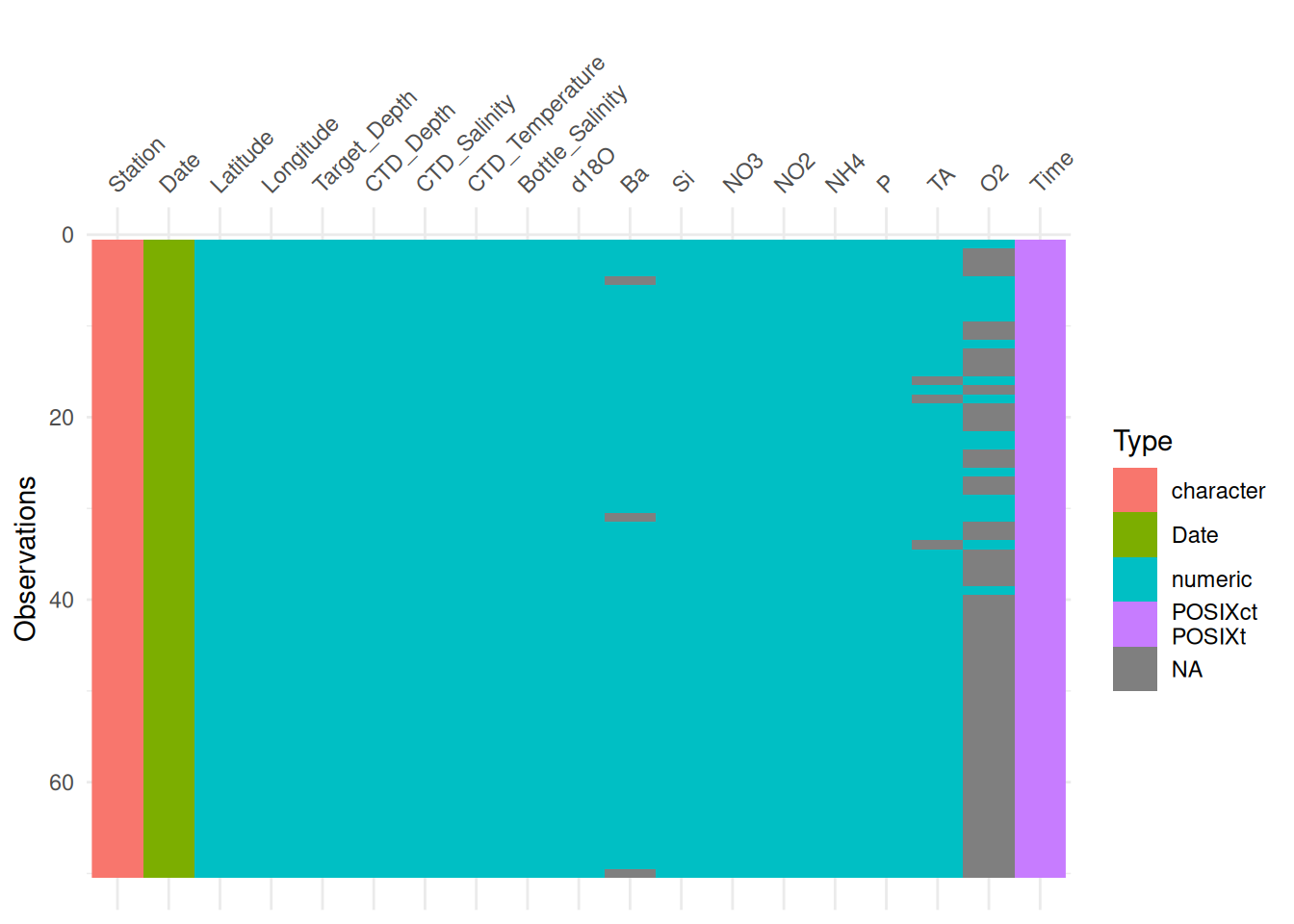
Similar to skimr, you can also group (in this case facet) the output by a variable.
vis_dat(bg_chem_clean, facet = Station) +
    theme(axis.text.x = element_text(angle = 45, vjust = 0))
This is helpful because it shows us where the missing values are and in which variable.
13.1.2.3 Formalized Validation with pointblank
library(pointblank)The pointblank package allows you to assess the state of data quality for a table according to a set of a priori rules that are user defined. Functions from the package integrate seamlessly into a tidyverse style workflow.
First we’ll show a simple example with our original bg_chem data. Here, we pipe bg_chem into the function col_vals_gt. The pointblank package has many, many different validation functions. For now, we’ll have a look at the col_vals_* family of functions, which check that values in the columns you declare meet some condition. In this example, we’ll use col_vals_gt to check that column values are greater than 0 by passing the columns to check to columns, and then to the value argument we pass 0 (what the values should be greater than). We can also specify whether NA values are allowed. The default there is FALSE so we will set to TRUE.
bg_chem %>%
    col_vals_gt(columns = O2, value = 0, na_pass = TRUE)
When we run this, you’ll see we get an error!
Error: Exceedance of failed test units where values in `O2` should have been > `0`.
The `col_vals_gt()` validation failed beyond the absolute threshold level (1).
* failure level (53) >= failure threshold (1)
And we expected this, we already knew this particular data frame had the -99 values in the O2 column. What the function did, then, was completely stop processing since the validation did not pass. This means that you can use these functions within data processing pipelines as ways to check and ensure your data are of high quality at key steps. For example, say our processing required us to transform this O2 variable in some way. You could add a validation step prior to a key mutate call to make sure that errors do not propogate through your data processing and analysis pipelines.
bg_chem_final <- bg_chem %>%
    col_vals_gt(columns = O2, value = 0, na_pass = TRUE) %>%
    mutate(important_metric = O2 * 0.321)
Error: Exceedance of failed test units where values in `O2` should have been > `0`.
The `col_vals_gt()` validation failed beyond the absolute threshold level (1).
* failure level (53) >= failure threshold (1)The reason why this works becomes apparent if we run this test on the bg_chem_clean dataset instead (the dataset that has -99 accounted for as a missing value).
bg_chem_clean %>%
    col_vals_gt(columns = O2, value = 0, na_pass = TRUE) %>%
    head()
# A tibble: 6 × 19
Date Time Station Latitude Longitude Target_Depth
<date> <dttm> <chr> <dbl> <dbl> <dbl>
1 2008-03-21 1899-12-31 21:56:46 73N,140W 73.0 -140. 20
2 2008-03-21 1899-12-31 21:56:46 73N,140W 73.0 -140. 60
3 2008-03-21 1899-12-31 21:56:46 73N,140W 73.0 -140. 85
4 2008-03-21 1899-12-31 21:56:46 73N,140W 73.0 -140. 190
5 2008-03-21 1899-12-31 21:56:46 73N,140W 73.0 -140. 310
6 2008-03-22 1899-12-31 21:45:27 72N,140W 72.1 -140. 20
# ℹ 13 more variables: CTD_Depth <dbl>, CTD_Salinity <dbl>,
# CTD_Temperature <dbl>, Bottle_Salinity <dbl>, d18O <dbl>, Ba <dbl>,
# Si <dbl>, NO3 <dbl>, NO2 <dbl>, NH4 <dbl>, P <dbl>, TA <dbl>, O2 <dbl>You’ll see from the above that if the test passes, the return value is just the data frame. So we can easily pipe it through to our important mutate call with no changes.
bg_chem_final <- bg_chem_clean %>%
    col_vals_gt(columns = O2, value = 0, na_pass = TRUE) %>%
    mutate(important_metric = O2 * 0.321)
13.1.2.3.1 Validation Reporting
pointblank also allows you to build a validation table, if, instead of inserting validation steps into processing pipelines, you just want to report on the quality of a particular data frame. To create this report, first we will use the create_agent function. This function takes the data.frame as an argument. After create_agent we pipe our validation functions like col_vals_gt above. Then, at the end, we pass those results to interrogate().
In this example, I will add more validation functions to different variables, and our agent and interrogation steps that generate a report:
bg_chem_clean %>%
    create_agent() %>%
    col_vals_gt(vars(O2, NO3, NO2, NH4, P, Si), value = 0, na_pass = TRUE) %>%
    col_vals_between(columns = vars(CTD_Salinity, Bottle_Salinity), left = 0, right = 42, na_pass = TRUE) %>%
    col_vals_between(Latitude, left = -90, right = 90) %>%
    col_vals_between(Longitude, left = -180, right = 180) %>%
interrogate()![]()
In the generated report, the left side of the table (red) shows the validation rules that were implemented. The right side shows the results. You can see that two of our rules, the greater than 0 rules for NO3 and NO2 has failures (in the FAIL column).
pointblank also allows you to set what are called action_levels. These signal thresholds for the following actions: warn, stop, and notify (W, S, N, respectively, in the right side of the validation table). These thresholds can be set as the relative proportion of failing rows or the absolute number of rows.
Let’s create some action levels so that we are warned 1 row failing, and stopped if more than 10.
al <- action_levels(warn_at = 1, stop_at = 10)We can then pass those action levels to the create_agent function to apply them to all of the rules.
bg_chem_clean %>%
    create_agent(actions = al) %>%
    col_vals_gt(vars(O2, NO3, NO2, NH4, P, Si), value = 0, na_pass = TRUE) %>%
    col_vals_between(columns = vars(CTD_Salinity, Bottle_Salinity), left = 0, right = 42, na_pass = TRUE) %>%
    col_vals_between(Latitude, left = -90, right = 90) %>%
    col_vals_between(Longitude, left = -180, right = 180) %>%
interrogate()You can also pass action levels to the validation functions themselves. Let’s say you want to have a different warning level for the lat/lons. We can override our less strict action level at the agent level at the lat/long validation step only.
al_latlon <- action_levels(warn_at = 1, stop_at = 5)bg_chem_clean %>%
create_agent(actions = al) %>%
col_vals_gt(vars(O2, NO3, NO2, NH4, P, Si), value = 0, na_pass = TRUE) %>%
col_vals_between(columns = vars(CTD_Salinity, Bottle_Salinity), left = 0, right = 42, na_pass = TRUE) %>%
col_vals_between(Latitude, left = -90, right = 90, actions = al_latlon) %>%
col_vals_between(Longitude, left = -180, right = 180, actions = al_latlon) %>%
interrogate()13.1.3 Summary
To summarize, we first talked about data quality as a concept. Data quality is not just “are my measurements valid?” - it also asks questions like:
- Are my files written according to their standard?
- Are my files documented accurately?
- Is my file encoded correctly?
We explored the Arctic Data Center’s automated data quality tools which seek to evaluate questions like those for all of the datasets at the Arctic Data Center.
Next, we showed how to evaluate data quality in R. Beginning with the humble file command, we expanded to look at two useful data summary packages, skimr and visdat which can help researchers spot quality issues quickly. Finally, we took a more in depth look at the pointblank package, which allows users to write their own data quality rules to either ensure that data look as expected through data processing operations, or to write a data quality report.