5 Session 5: Cleaning and Manipulating Data
5.1 Data Cleaning and Manipulation
5.1.1 Learning Objectives
In this lesson, you will learn:
- What the Split-Apply-Combine strategy is and how it applies to data
- The difference between wide vs. tall table formats and how to convert between them
- How to use
dplyrandtidyrto clean and manipulate data for analysis - How to join multiple
data.frames together usingdplyr
5.1.2 Introduction
The data we get to work with are rarely, if ever, in the format we need to do our analyses. It’s often the case that one package requires data in one format, while another package requires the data to be in another format. To be efficient analysts, we should have good tools for reformatting data for our needs so we can do our actual work like making plots and fitting models. The dplyr and tidyr R packages provide a fairly complete and extremely powerful set of functions for us to do this reformatting quickly and learning these tools well will greatly increase your efficiency as an analyst.
Analyses take many shapes, but they often conform to what is known as the Split-Apply-Combine strategy. This strategy follows a usual set of steps:
- Split: Split the data into logical groups (e.g., area, stock, year)
- Apply: Calculate some summary statistic on each group (e.g. mean total length by year)
- Combine: Combine the groups back together into a single table
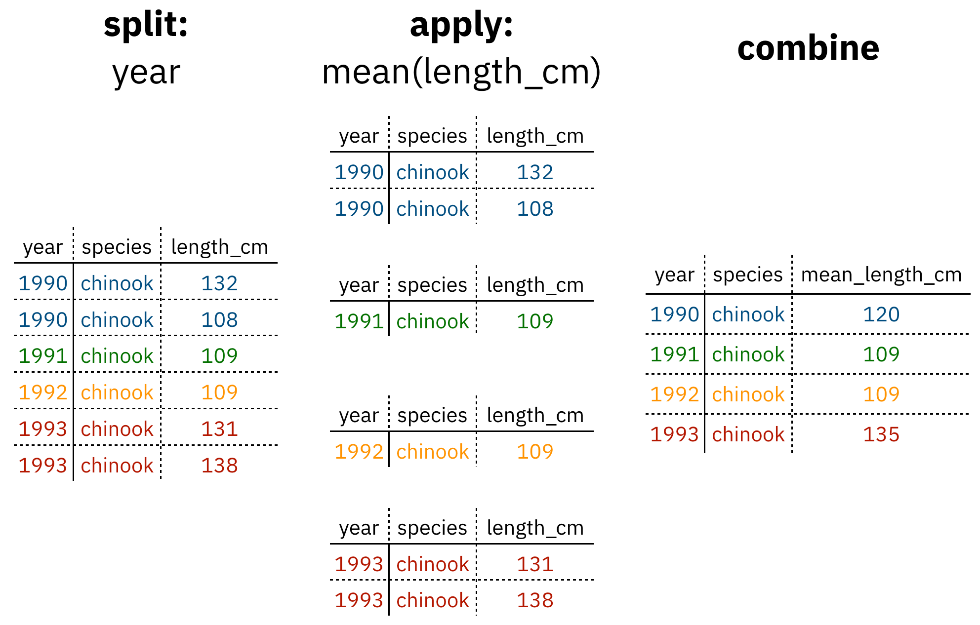
Figure 1: diagram of the split apply combine strategy
As shown above (Figure 1), our original table is split into groups by year, we calculate the mean length for each group, and finally combine the per-year means into a single table.
dplyr provides a fast and powerful way to express this. Let’s look at a simple example of how this is done:
Assuming our length data is already loaded in a data.frame called length_data:
| year | length_cm |
|---|---|
| 1991 | 5.673318 |
| 1991 | 3.081224 |
| 1991 | 4.592696 |
| 1992 | 4.381523 |
| 1992 | 5.597777 |
| 1992 | 4.900052 |
| 1992 | 4.139282 |
| 1992 | 5.422823 |
| 1992 | 5.905247 |
| 1992 | 5.098922 |
We can do this calculation using dplyr like this:
length_data %>%
  group_by(year) %>%
  summarise(mean_length_cm = mean(length_cm))
Another exceedingly common thing we need to do is “reshape” our data. Let’s look at an example table that is in what we will call “wide” format:
| site | 1990 | 1991 | … | 1993 |
|---|---|---|---|---|
| gold | 100 | 118 | … | 112 |
| lake | 100 | 118 | … | 112 |
| … | … | … | … | … |
| dredge | 100 | 118 | … | 112 |
You are probably quite familiar with data in the above format, where values of the variable being observed are spread out across columns (Here: columns for each year). Another way of describing this is that there is more than one measurement per row. This wide format works well for data entry and sometimes works well for analysis but we quickly outgrow it when using R. For example, how would you fit a model with year as a predictor variable? In an ideal world, we’d be able to just run:
lm(length ~ year)But this won’t work on our wide data because lm needs length and year to be columns in our table.
Or how would we make a separate plot for each year? We could call plot one time for each year but this is tedious if we have many years of data and hard to maintain as we add more years of data to our dataset.
The tidyr package allows us to quickly switch between wide format and what is called tall format using the pivot_longer function:
site_data %>%
pivot_longer(-site, names_to = "year", values_to = "length")| site | year | length |
|---|---|---|
| gold | 1990 | 101 |
| lake | 1990 | 104 |
| dredge | 1990 | 144 |
| … | … | … |
| dredge | 1993 | 145 |
In this lesson we’re going to walk through the functions you’ll most commonly use from the dplyr and tidyr packages:
dplyrmutate()group_by()summarise()select()filter()arrange()left_join()rename()
tidyrpivot_longer()pivot_wider()unite()separate()
5.1.3 Data Cleaning Basics
To demonstrate, we’ll be working with a tidied up version of a dataset from ADF&G containing commercial catch data from 1878-1997. The dataset and reference to the original source can be found at its public archive: https://knb.ecoinformatics.org/#view/df35b.304.2.
First, open a new RMarkdown document. Delete everything below the setup chunk, and add a library chunk that calls dplyr, tidyr, and readr:
library(dplyr)
library(tidyr)
library(readr)
Aside
A note on loading packages.
You may have noticed the following warning messages pop up when you ran your library chunk.
Attaching package: ‘dplyr’

The following objects are masked from ‘package:stats’:

    filter, lag

The following objects are masked from ‘package:base’:

    intersect, setdiff, setequal, union
These are important warnings. They are letting you know that certain functions from the stats and base packages (which are loaded by default when you start R) are masked by different functions with the same name in the dplyr package. It turns out, the order that you load the packages in matters. Since we loaded dplyr after stats, R will assume that if you call filter, you mean the dplyr version unless you specify otherwise.
Being specific about which version of filter, for example, you call is easy. To explicitly call a function by its unambiguous name, you use the syntax package_name::function_name(...). So, if I wanted to call the stats version of filter in this Rmarkdown document, I would use the syntax stats::filter(...).
Challenge
The warnings above are important, but we might not want them in our final document. After you have read them, adjust the chunk settings on your library chunk to suppress warnings and messages.
Now that we have learned a little mini-lesson on functions, let’s get the data that we are going to use for this lesson.
Setup
Navigate to the salmon catch dataset: https://knb.ecoinformatics.org/#view/df35b.304.2
Right click the “download” button for the file “byerlySalmonByRegion.csv”
Select “copy link address” from the dropdown menu
Paste the URL into a
read.csvcall like below
The code chunk you use to read in the data should look something like this:
catch_original <- read.csv("https://knb.ecoinformatics.org/knb/d1/mn/v2/object/df35b.302.1")Aside
Note that windows users who want to use this method locally also need to use the url function here with the argument method = "libcurl" as below:
catch_original <- read.csv(url("https://knb.ecoinformatics.org/knb/d1/mn/v2/object/df35b.302.1", method = "libcurl"))This dataset is relatively clean and easy to interpret as-is. But while it may be clean, it’s in a shape that makes it hard to use for some types of analyses so we’ll want to fix that first.
Challenge
Before we get too much further, spend a minute or two outlining your RMarkdown document so that it includes the following sections and steps:
- Data Sources
- read in the data
- Clean and Reshape data
- remove unnecessary columns
- check column typing
- reshape data
- Join to Regions dataset
About the pipe (%>%) operator
Before we jump into learning tidyr and dplyr, we first need to explain the %>%.
Both the tidyr and the dplyr packages use the pipe operator - %>%, which may look unfamiliar. The pipe is a powerful way to efficiently chain together operations. The pipe will take the output of a previous statement, and use it as the input to the next statement.
Say you want to both filter out rows of a dataset, and select certain columns. Instead of writing
df_filtered <- filter(df, ...)
df_selected <- select(df_filtered, ...)
You can write
df_cleaned <- df %>%
              filter(...) %>%
              select(...)
If you think of the assignment operator (<-) as reading like “gets,” then the pipe operator would read like “then.”
So you might think of the above chunk being translated as:
The cleaned dataframe gets the original data, and then a filter (of the original data), and then a select (of the filtered data).
The benefits to using pipes are that you don’t have to keep track of (or overwrite) intermediate data frames. The drawbacks are that it can be more difficult to explain the reasoning behind each step, especially when many operations are chained together. It is good to strike a balance between writing efficient code (chaining operations), while ensuring that you are still clearly explaining, both to your future self and others, what you are doing and why you are doing it.
RStudio has a keyboard shortcut for %>% : Ctrl + Shift + M (Windows), Cmd + Shift + M (Mac).
Selecting/removing columns: select()
The first issue is the extra columns All and notesRegCode. Let’s select only the columns we want, and assign this to a variable called catch_data.
catch_data <- catch_original %>%
  select(Region, Year, Chinook, Sockeye, Coho, Pink, Chum)

head(catch_data)
## Region Year Chinook Sockeye Coho Pink Chum
## 1 SSE 1886 0 5 0 0 0
## 2 SSE 1887 0 155 0 0 0
## 3 SSE 1888 0 224 16 0 0
## 4 SSE 1889 0 182 11 92 0
## 5 SSE 1890 0 251 42 0 0
## 6 SSE 1891 0 274 24 0 0Much better!
select also allows you to say which columns you don’t want, by passing unquoted column names preceded by minus (-) signs:
catch_data <- catch_original %>%
  select(-All, -notesRegCode)

head(catch_data)
Quality Check
Now that we have the data we are interested in using, we should do a little quality check to see that it seems as expected. One nice way of doing this is the glimpse function.
glimpse(catch_data)## Rows: 1,708
## Columns: 7
## $ Region <chr> "SSE", "SSE", "SSE", "SSE", "SSE", "SSE", "SSE", "SSE", "SSE", "SSE", "SSE", "SSE", "SSE", "SSE", "SSE", "SSE", "SS…
## $ Year <int> 1886, 1887, 1888, 1889, 1890, 1891, 1892, 1893, 1894, 1895, 1896, 1897, 1898, 1899, 1900, 1901, 1902, 1903, 1904, 1…
## $ Chinook <chr> "0", "0", "0", "0", "0", "0", "0", "0", "0", "3", "4", "5", "9", "12", "0", "3", "4", "0", "4", "9", "3", "17", "43…
## $ Sockeye <int> 5, 155, 224, 182, 251, 274, 207, 189, 253, 408, 989, 791, 708, 797, 763, 264, 256, 230, 1143, 1009, 981, 808, 731, …
## $ Coho <int> 0, 0, 16, 11, 42, 24, 11, 1, 5, 8, 192, 161, 132, 139, 84, 107, 34, 125, 242, 184, 169, 180, 186, 128, 235, 355, 51…
## $ Pink <int> 0, 0, 0, 92, 0, 0, 8, 187, 529, 606, 996, 2218, 673, 1545, 2040, 1049, 1547, 669, 2381, 2060, 3859, 8055, 7120, 678…
## $ Chum <int> 0, 0, 0, 0, 0, 0, 0, 0, 0, 0, 0, 7, 0, 1, 2, 0, 0, 0, 102, 343, 473, 437, 616, 249, 1121, 1141, 2685, 1384, 3783, 2…Challenge
Notice the output of the glimpse function call. Does anything seem amiss with this dataset that might warrant fixing?
Answer:
The Chinook catch data arecharacter class. Let’s fix it using the function mutate before moving on.
Changing column content: mutate()
We can use the mutate function to change a column, or to create a new column. First Let’s try to just convert the Chinook catch values to numeric type using the as.numeric() function, and overwrite the old Chinook column.
catch_clean <- catch_data %>%
  mutate(Chinook = as.numeric(Chinook))
## Warning in mask$eval_all_mutate(quo): NAs introduced by coercionhead(catch_clean)## Region Year Chinook Sockeye Coho Pink Chum
## 1 SSE 1886 0 5 0 0 0
## 2 SSE 1887 0 155 0 0 0
## 3 SSE 1888 0 224 16 0 0
## 4 SSE 1889 0 182 11 92 0
## 5 SSE 1890 0 251 42 0 0
## 6 SSE 1891 0 274 24 0 0We get a warning “NAs introduced by coercion” which is R telling us that it couldn’t convert every value to an integer and, for those values it couldn’t convert, it put an NA in its place. This is behavior we commonly experience when cleaning datasets and it’s important to have the skills to deal with it when it crops up.
To investigate, let’s isolate the issue. We can find out which values are NAs with a combination of is.na() and which(), and save that to a variable called i.
i <- which(is.na(catch_clean$Chinook))
i
## [1] 401It looks like there is only one problem row, lets have a look at it in the original data.
catch_data[i,]## Region Year Chinook Sockeye Coho Pink Chum
## 401 GSE 1955 I 66 0 0 1Well that’s odd: The value in catch_thousands is I. It turns out that this dataset is from a PDF which was automatically converted into a CSV and this value of I is actually a 1.
Let’s fix it by incorporating the ifelse function to our mutate call, which will change the value of the Chinook column to 1 if the value is equal to I, otherwise it will use as.numeric to turn the character representations of numbers into numeric typed values.
catch_clean <- catch_data %>%
  mutate(Chinook = if_else(Chinook == "I", "1", Chinook)) %>%
  mutate(Chinook = as.integer(Chinook))

head(catch_clean)
## Region Year Chinook Sockeye Coho Pink Chum
## 1 SSE 1886 0 5 0 0 0
## 2 SSE 1887 0 155 0 0 0
## 3 SSE 1888 0 224 16 0 0
## 4 SSE 1889 0 182 11 92 0
## 5 SSE 1890 0 251 42 0 0
## 6 SSE 1891 0 274 24 0 0Changing shape: pivot_longer() and pivot_wider()
The next issue is that the data are in a wide format and, we want the data in a tall format instead. pivot_longer() from the tidyr package helps us do just this conversion:
catch_long <- catch_clean %>%
  pivot_longer(cols = -c(Region, Year), names_to = "species", values_to = "catch")

head(catch_long)
## # A tibble: 6 × 4
## Region Year species catch
## <chr> <int> <chr> <int>
## 1 SSE 1886 Chinook 0
## 2 SSE 1886 Sockeye 5
## 3 SSE 1886 Coho 0
## 4 SSE 1886 Pink 0
## 5 SSE 1886 Chum 0
## 6 SSE 1887 Chinook 0The syntax we used above for pivot_longer() might be a bit confusing so let’s walk though it.
The first argument to pivot_longer is the columns over which we are pivoting. You can select these by listing either the names of the columns you do want to pivot, or the names of the columns you are not pivoting over. The names_to argument takes the name of the column that you are creating from the column names you are pivoting over. The values_to argument takes the name of the column that you are creating from the values in the columns you are pivoting over.
The opposite of pivot_longer(), pivot_wider(), works in a similar declarative fashion:
catch_wide <- catch_long %>%
  pivot_wider(names_from = species, values_from = catch)

head(catch_wide)
## # A tibble: 6 × 7
## Region Year Chinook Sockeye Coho Pink Chum
## <chr> <int> <int> <int> <int> <int> <int>
## 1 SSE 1886 0 5 0 0 0
## 2 SSE 1887 0 155 0 0 0
## 3 SSE 1888 0 224 16 0 0
## 4 SSE 1889 0 182 11 92 0
## 5 SSE 1890 0 251 42 0 0
## 6 SSE 1891 0 274 24 0 0Renaming columns with rename()
If you scan through the data, you may notice the values in the catch column are very small (these are supposed to be annual catches). If we look at the metadata we can see that the catch column is in thousands of fish so let’s convert it before moving on.
Let’s first rename the catch column to be called catch_thousands:
catch_long <- catch_long %>%
  rename(catch_thousands = catch)

head(catch_long)
## # A tibble: 6 × 4
## Region Year species catch_thousands
## <chr> <int> <chr> <int>
## 1 SSE 1886 Chinook 0
## 2 SSE 1886 Sockeye 5
## 3 SSE 1886 Coho 0
## 4 SSE 1886 Pink 0
## 5 SSE 1886 Chum 0
## 6 SSE 1887 Chinook 0Aside
Many people use the base R function names to rename columns, often in combination with column indexing that relies on columns being in a particular order. Column indexing is often also used to select columns instead of the select function from dplyr. Although these methods both work just fine, they do have one major drawback: in most implementations they rely on you knowing exactly the column order your data is in.
To illustrate why your knowledge of column order isn’t reliable enough for these operations, considering the following scenario:
Your colleague emails you letting you know that she has an updated version of the conductivity-temperature-depth data from this year’s research cruise, and sends it along. Excited, you re-run your scripts that use this data for your phytoplankton research. You run the script and suddenly all of your numbers seem off. You spend hours trying to figure out what is going on.
Unbeknownst to you, your colleagues bought a new sensor this year that measures dissolved oxygen. Because of the new variables in the dataset, the column order is different. Your script which previously renamed the 4th column, SAL_PSU to salinity now renames the 4th column, O2_MGpL to salinity. No wonder your results looked so weird, good thing you caught it!
If you had written your code so that it doesn’t rely on column order, but instead renames columns using the rename function, the code would have run just fine (assuming the name of the original salinity column didn’t change, in which case the code would have errored in an obvious way). This is an example of a defensive coding strategy, where you try to anticipate issues before they arise, and write your code in such a way as to keep the issues from happening.
Adding columns: mutate()
Now let’s use mutate again to create a new column called catch with units of fish (instead of thousands of fish).
catch_long <- catch_long %>%
  mutate(catch = catch_thousands * 1000)

head(catch_long)
Now let’s remove the catch_thousands column for now since we don’t need it. Note that here we have added to the expression we wrote above by adding another function call (mutate) to our expression. This takes advantage of the pipe operator by grouping together a similar set of statements, which all aim to clean up the catch_long data.frame.
catch_long <- catch_long %>%
  mutate(catch = catch_thousands * 1000) %>%
  select(-catch_thousands)

head(catch_long)
## # A tibble: 6 × 4
## Region Year species catch
## <chr> <int> <chr> <dbl>
## 1 SSE 1886 Chinook 0
## 2 SSE 1886 Sockeye 5000
## 3 SSE 1886 Coho 0
## 4 SSE 1886 Pink 0
## 5 SSE 1886 Chum 0
## 6 SSE 1887 Chinook 0We’re now ready to start analyzing the data.
group_by and summarise
As I outlined in the Introduction, dplyr lets us employ the Split-Apply-Combine strategy and this is exemplified through the use of the group_by() and summarise() functions:
mean_region <- catch_long %>%
  group_by(Region) %>%
  summarise(catch_mean = mean(catch))

head(mean_region)
## # A tibble: 6 × 2
## Region catch_mean
## <chr> <dbl>
## 1 ALU 40384.
## 2 BER 16373.
## 3 BRB 2709796.
## 4 CHG 315487.
## 5 CKI 683571.
## 6 COP 179223.Another common use of group_by() followed by summarize() is to count the number of rows in each group. We have to use a special function from dplyr, n().
n_region <- catch_long %>%
  group_by(Region) %>%
  summarize(n = n())

head(n_region)
## # A tibble: 6 × 2
## Region n
## <chr> <int>
## 1 ALU 435
## 2 BER 510
## 3 BRB 570
## 4 CHG 550
## 5 CKI 525
## 6 COP 470Aside
If you are finding that you are reaching for this combination of group_by(), summarise() and n() a lot, there is a helpful dplyr function count() that accomplishes this in one function!
Challenge
- Find another grouping and statistic to calculate for each group.
- Find out if you can group by multiple variables.
Filtering rows: filter()
filter() is the verb we use to filter our data.frame to rows matching some condition. It’s similar to subset() from base R.
Let’s go back to our original data.frame and do some filter()ing:
SSE_catch <- catch_long %>%
  filter(Region == "SSE")

head(SSE_catch)
## # A tibble: 6 × 4
## Region Year species catch
## <chr> <int> <chr> <dbl>
## 1 SSE 1886 Chinook 0
## 2 SSE 1886 Sockeye 5000
## 3 SSE 1886 Coho 0
## 4 SSE 1886 Pink 0
## 5 SSE 1886 Chum 0
## 6 SSE 1887 Chinook 0Challenge
- Filter to just catches of over one million fish.
- Filter to just Chinook from the SSE region
Sorting your data: arrange()
arrange() is how we sort the rows of a data.frame. In my experience, I use arrange() in two common cases:
- When I want to calculate a cumulative sum (with
cumsum()) so row order matters - When I want to display a table (like in an
.Rmddocument) in sorted order
Let’s re-calculate mean catch by region, and then arrange() the output by mean catch:
mean_region <- catch_long %>%
  group_by(Region) %>%
  summarise(mean_catch = mean(catch)) %>%
  arrange(mean_catch)

head(mean_region)
## # A tibble: 6 × 2
## Region mean_catch
## <chr> <dbl>
## 1 BER 16373.
## 2 KTZ 18836.
## 3 ALU 40384.
## 4 NRS 51503.
## 5 KSK 67642.
## 6 YUK 68646.The default sorting order of arrange() is to sort in ascending order. To reverse the sort order, wrap the column name inside the desc() function:
mean_region <- catch_long %>%
  group_by(Region) %>%
  summarise(mean_catch = mean(catch)) %>%
  arrange(desc(mean_catch))

head(mean_region)
## # A tibble: 6 × 2
## Region mean_catch
## <chr> <dbl>
## 1 SSE 3184661.
## 2 BRB 2709796.
## 3 NSE 1825021.
## 4 KOD 1528350
## 5 PWS 1419237.
## 6 SOP 1110942.5.1.4 Joins in dplyr
So now that we’re awesome at manipulating a single data.frame, where do we go from here? Manipulating more than one data.frame.
If you’ve ever used a database, you may have heard of or used what’s called a “join,” which allows us to to intelligently merge two tables together into a single table based upon a shared column between the two. We’ve already covered joins in Data Modeling & Tidy Data so let’s see how it’s done with dplyr.
The dataset we’re working with, https://knb.ecoinformatics.org/#view/df35b.304.2, contains a second CSV which has the definition of each Region code. This is a really common way of storing auxiliary information about our dataset of interest (catch) but, for analylitcal purposes, we often want them in the same data.frame. Joins let us do that easily.
Let’s look at a preview of what our join will do by looking at a simplified version of our data:
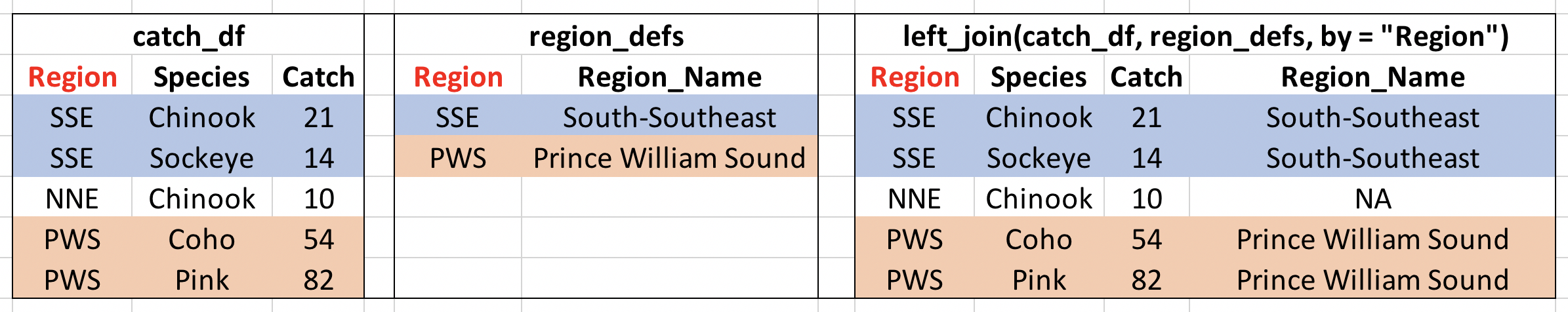
Visualisation of our left_join
First, let’s read in the region definitions data table and select only the columns we want. Note that I have piped my read.csv result into a select call, creating a tidy chunk that reads and selects the data that we need.
region_defs <- read.csv("https://knb.ecoinformatics.org/knb/d1/mn/v2/object/df35b.303.1") %>%
    select(code, mgmtArea)

head(region_defs)
## code mgmtArea
## 1 GSE Unallocated Southeast Alaska
## 2 NSE Northern Southeast Alaska
## 3 SSE Southern Southeast Alaska
## 4 YAK Yakutat
## 5 PWSmgmt Prince William Sound Management Area
## 6 BER Bering River Subarea Copper River SubareaIf you examine the region_defs data.frame, you’ll see that the column names don’t exactly match the image above. If the names of the key columns are not the same, you can explicitly specify which are the key columns in the left and right side as shown below:
catch_joined <- left_join(catch_long, region_defs, by = c("Region" = "code"))

head(catch_joined)
## # A tibble: 6 × 5
## Region Year species catch mgmtArea
## <chr> <int> <chr> <dbl> <chr>
## 1 SSE 1886 Chinook 0 Southern Southeast Alaska
## 2 SSE 1886 Sockeye 5000 Southern Southeast Alaska
## 3 SSE 1886 Coho 0 Southern Southeast Alaska
## 4 SSE 1886 Pink 0 Southern Southeast Alaska
## 5 SSE 1886 Chum 0 Southern Southeast Alaska
## 6 SSE 1887 Chinook 0 Southern Southeast AlaskaNotice that I have deviated from our usual pipe syntax (although it does work here!) because I prefer to see the data.frames that I am joining side by side in the syntax.
Another way you can do this join is to use rename to change the column name code to Region in the region_defs data.frame, and run the left_join this way:
region_defs <- region_defs %>%
  rename(Region = code, Region_Name = mgmtArea)

catch_joined <- left_join(catch_long, region_defs, by = c("Region"))

head(catch_joined)
Now our catches have the auxiliary information from the region definitions file alongside them. Note: dplyr provides a complete set of joins: inner, left, right, full, semi, anti, not just left_join.
separate() and unite()
separate() and its complement, unite() allow us to easily split a single column into numerous (or numerous into a single).
This can come in really handle when we need to split a column into two pieces by a consistent separator (like a dash).
Let’s make a new data.frame with fake data to illustrate this. Here we have a set of site identification codes. with information about the island where the site is (the first 3 letters) and a site number (the 3 numbers). If we want to group and summarize by island, we need a column with just the island information.
sites_df <- data.frame(site = c("HAW-101",
                                "HAW-103",
                                "OAH-320",
                                "OAH-219",
                                "MAI-039"))

sites_df %>%
  separate(site, c("island", "site_number"), "-")
## island site_number
## 1 HAW 101
## 2 HAW 103
## 3 OAH 320
## 4 OAH 219
## 5 MAI 039- Exercise: Split the
citycolumn in the followingdata.frameintocityandstate_codecolumns:
cities_df <- data.frame(city = c("Juneau AK",
                                 "Sitka AK",
                                 "Anchorage AK"))

# Write your solution here
unite() does just the reverse of separate(). If we have a data.frame that contains columns for year, month, and day, we might want to unite these into a single date column.
dates_df <- data.frame(year = c("1930",
                                "1930",
                                "1930"),
                       month = c("12",
                                "12",
                                "12"),
                       day = c("14",
                               "15",
                               "16"))

dates_df %>%
  unite(date, year, month, day, sep = "-")
## date
## 1 1930-12-14
## 2 1930-12-15
## 3 1930-12-16- Exercise: Use
unite()on your solution above to combine thecities_dfback to its original form with just one column,city:
# Write your solution hereSummary
We just ran through the various things we can do with dplyr and tidyr but if you’re wondering how this might look in a real analysis. Let’s look at that now:
catch_original <- read.csv(url("https://knb.ecoinformatics.org/knb/d1/mn/v2/object/df35b.302.1", method = "libcurl"))
region_defs <- read.csv(url("https://knb.ecoinformatics.org/knb/d1/mn/v2/object/df35b.303.1", method = "libcurl")) %>%
    select(code, mgmtArea)

mean_region <- catch_original %>%
  select(-All, -notesRegCode) %>%
  mutate(Chinook = ifelse(Chinook == "I", 1, Chinook)) %>%
  mutate(Chinook = as.numeric(Chinook)) %>%
  pivot_longer(-c(Region, Year), names_to = "species", values_to = "catch") %>%
  mutate(catch = catch*1000) %>%
  group_by(Region) %>%
  summarize(mean_catch = mean(catch)) %>%
  left_join(region_defs, by = c("Region" = "code"))

head(mean_region)
## # A tibble: 6 × 3
## Region mean_catch mgmtArea
## <chr> <dbl> <chr>
## 1 ALU 40384. Aleutian Islands Subarea
## 2 BER 16373. Bering River Subarea Copper River Subarea
## 3 BRB 2709796. Bristol Bay Management Area
## 4 CHG 315487. Chignik Management Area
## 5 CKI 683571. Cook Inlet Management Area
## 6 COP 179223. Copper River Subarea