6 Data Modeling Essentials

Learning Objectives

• Review high level best practices for effective data management
• Understand the principles of tidy data
• Introduce the relational data model
• Learn how to design and diagram multi-table data models

6.1 Simple guidelines for data management

A great paper called ‘Some Simple Guidelines for Effective Data Management’ (Borer et al. 2009) lays out exactly that - guidelines that make your data management, and your reproducible research, more effective. Although not strictly about data modeling, the first six guidelines are worth remembering as foundational guidelines, here slightly revised to reflect changes over the intervening years:

Use a scripted workflow

Manipulating data using scripts (like R!) gives you much more control over all decisions and changes. Scripts allow you to document, audit, edit, reuse, and reproduce all steps. In contrast, point-and-click manipulations, such as manually editing data in a spreadsheet application, are time consuming, poorly documented, and difficult to reproduce.

Keep a raw version of data

In conjunction with using a scripted language, keeping a raw version of your data is essential for maintaining a reproducible workflow. When you keep your raw data, your scripts can read from that raw data and create as many derived data products as you need, and you will always be able to re-run your scripts and know that you will get the same output.

Prefer open file formats (e.g. csv, txt)

Using a file that can be read by free, open source software greatly increases the longevity and accessibility of your data. In contrast, proprietary formats bind your data to a particular vendor or software license that may be hard to maintain and may become obsolete.

Use simple but descriptive names

File and variable names should be descriptive, helping your future self and others more quickly understand what type of data they contain, but also simple - in particular, without spaces or special characters - to reduce issues when reading and referring to them in scripts and other programmatic environments.

Include a header line in your data tables

When creating and managin tabular data, using a single header line of column names as the first row of your table is the most common and easiest way to achieve consistency among files.

Use plain ASCII or UTF-8 for text

Standard character encodings such as ASCII and UTF-8 are widely used for text files, hence far more likely to be parsed correctly and supported well into the future as compared with more esoteric formats.

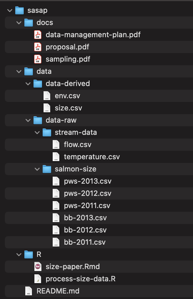
Before moving on to discuss the remaining guidelines, here is an example of how you might organize the files themselves following the simple rules above. Note that we have all open formats, plain text formats for data, sortable file names without special characters, scripts, and a special folder for raw files.

6.2 Tidy data

The final 3 guidelines focus on the structural design of data tables:

• Design tables to add rows, not columns
• Each column should contain only one type of information
• Record a single piece of data only once; separate information collected at different scales into different tables.

More recently, these have been popularized under the tidy data principles, which articulate a simple but effective pattern for organizing data tables in a way that allows us to understand, manage, and analyze data efficiently:

1. Every column is a variable.
2. Every row is an observation.
3. Every cell is a single value.

Why Tidy Data?

• Efficiency: less re-creating the wheel. Easier to apply the same tools to different datasets.
• Collaboration: Makes it easier to work with others as you can work with the same tools in the same ways.
• Reuse: It makes it easier to apply similar techniques and analysis across different or new datasets.
• Generalizability: Tools built for one tidy data set can be used to multiple other datasets. Opening posibilities of data you can work with.

“There is a specific advantage to placing varables in columns becasuse it allows R’s vectorized nature to shine. …most buit-in R functions work with vactors of values. That makes transforming tidy data feel particularly natural.” (R for Data Science by Grolemund and Wickham)

Tidy Data: A way of life

• Tidy data is not a language or tool specific.
• Tidy data is not an R thing.
• Tidy data is not a tidyverse thing.

Tidy Data is a way to organize data that will make life easier for people working with data.

(Allison Horst & Julia Lowndes)

Let’s make sure we understand the basic terms used above, along with a fourth term (“entity”) that we’ll discuss more later.

Concept	Definition
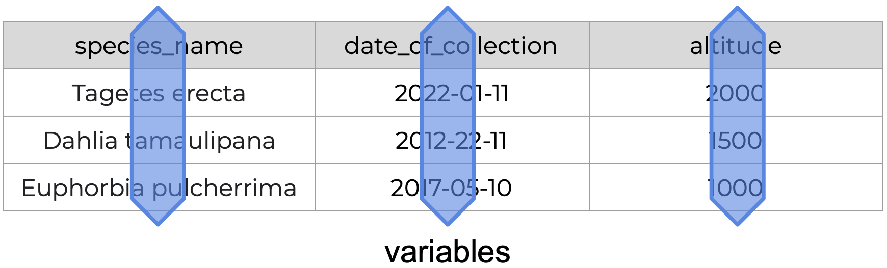
Variables	A characteristic that is being measured, counted, or described with data. Example: car type, salinity, year, height, mass.
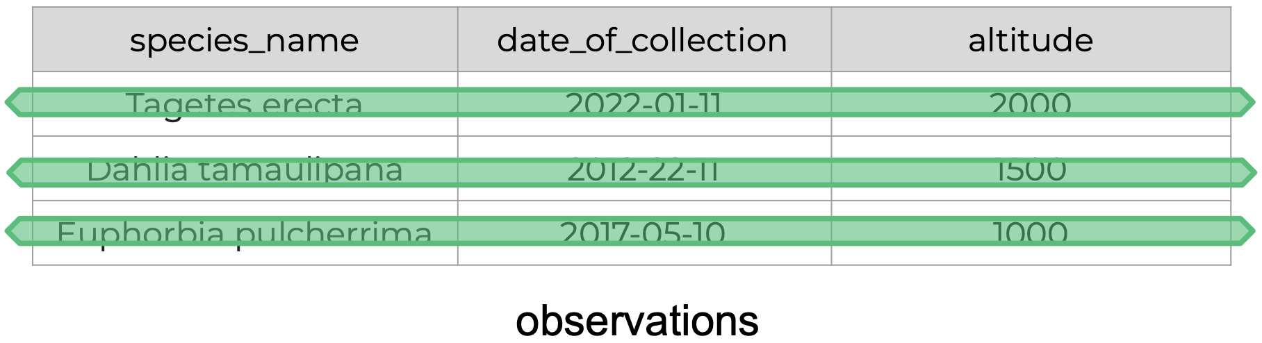
Observations	A single “data point” for which the measure, count, or description of one or more variables is recorded. Example: If you are collecting variables height, species, and location of plants, then each plant is an observation.
Value	The record measured, count, or description of a variable. Example: 3 ft
Entity	Each type of observation is an entity. Example: If you are recording the species name and height of plants observed at various sites that each have a site name and location, then plants is an entity and site is an entity.

6.2.1 Tidy data in action

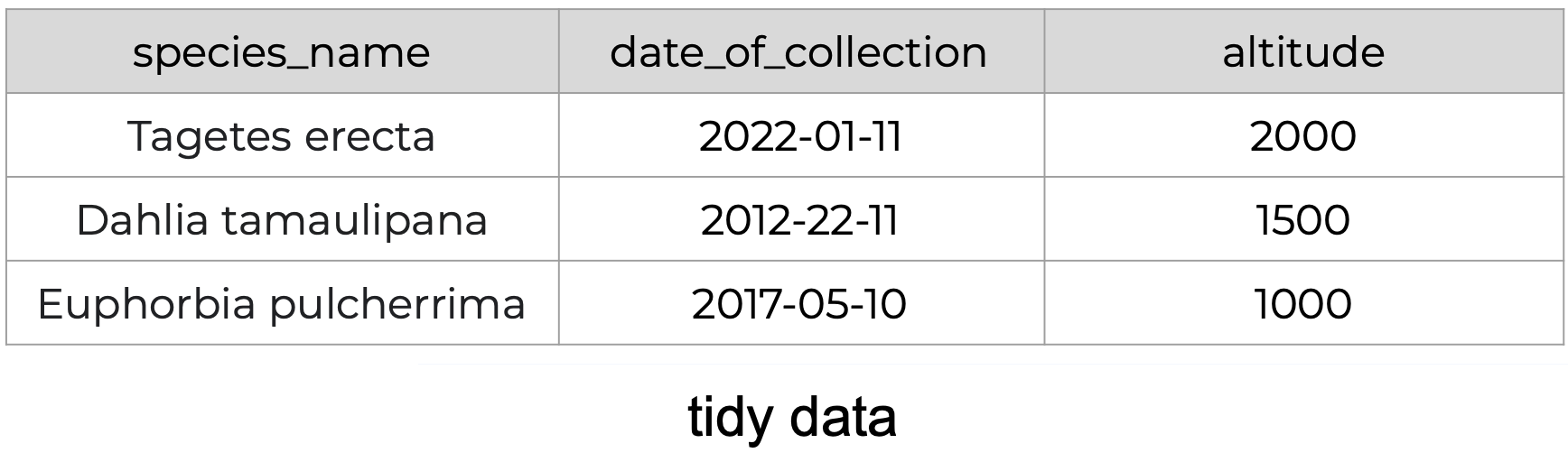
The following is an example of tidy data - it’s easy to see the three tidy data principles apply.

6.2.2 Recognizing untidy data

Anything that does not follow the three tidy data principles is untidy data.

There are many ways in which data can become untidy. Some are obvious once you know what to look for, while others are more subtle. In this section we will look at some examples of common untidy data situations.

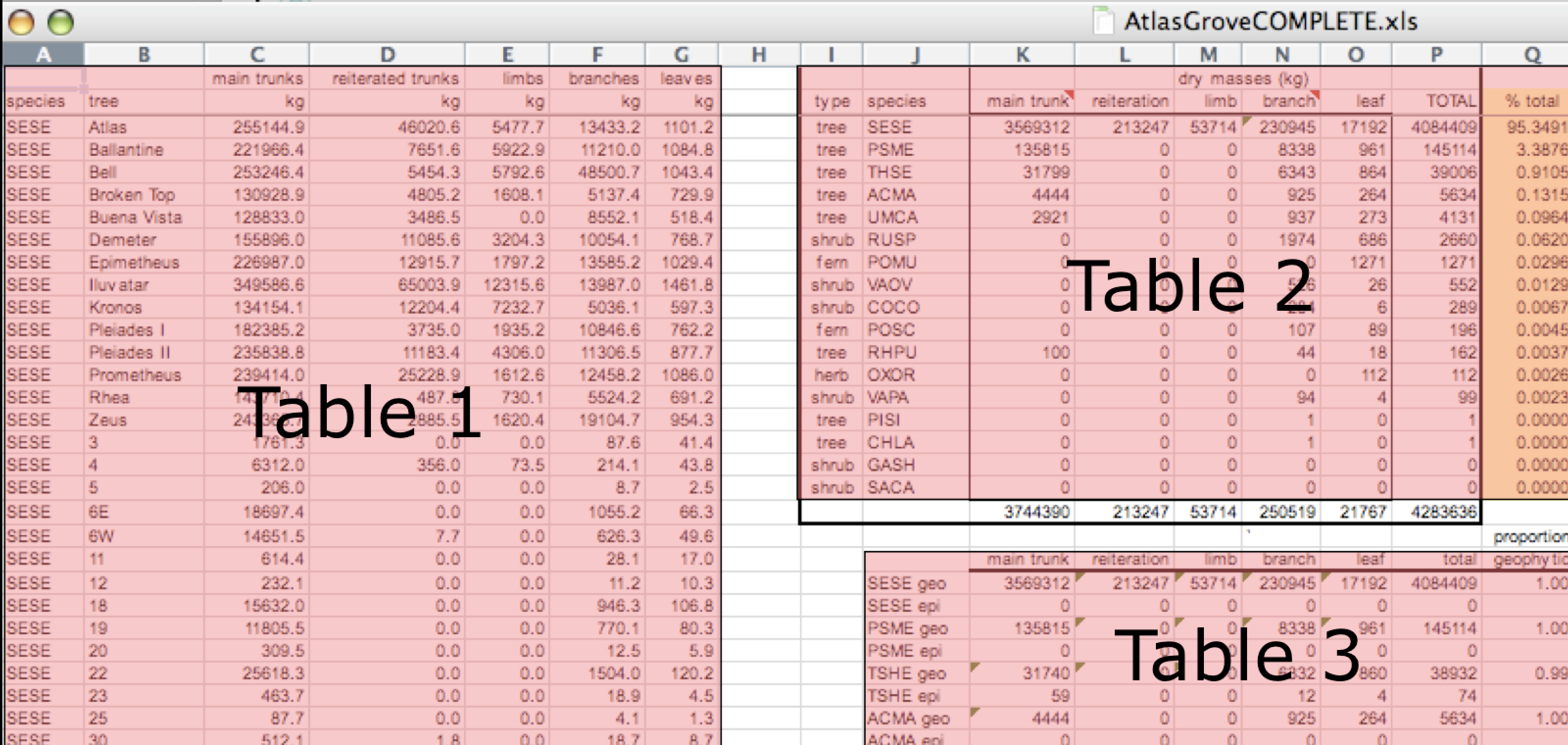
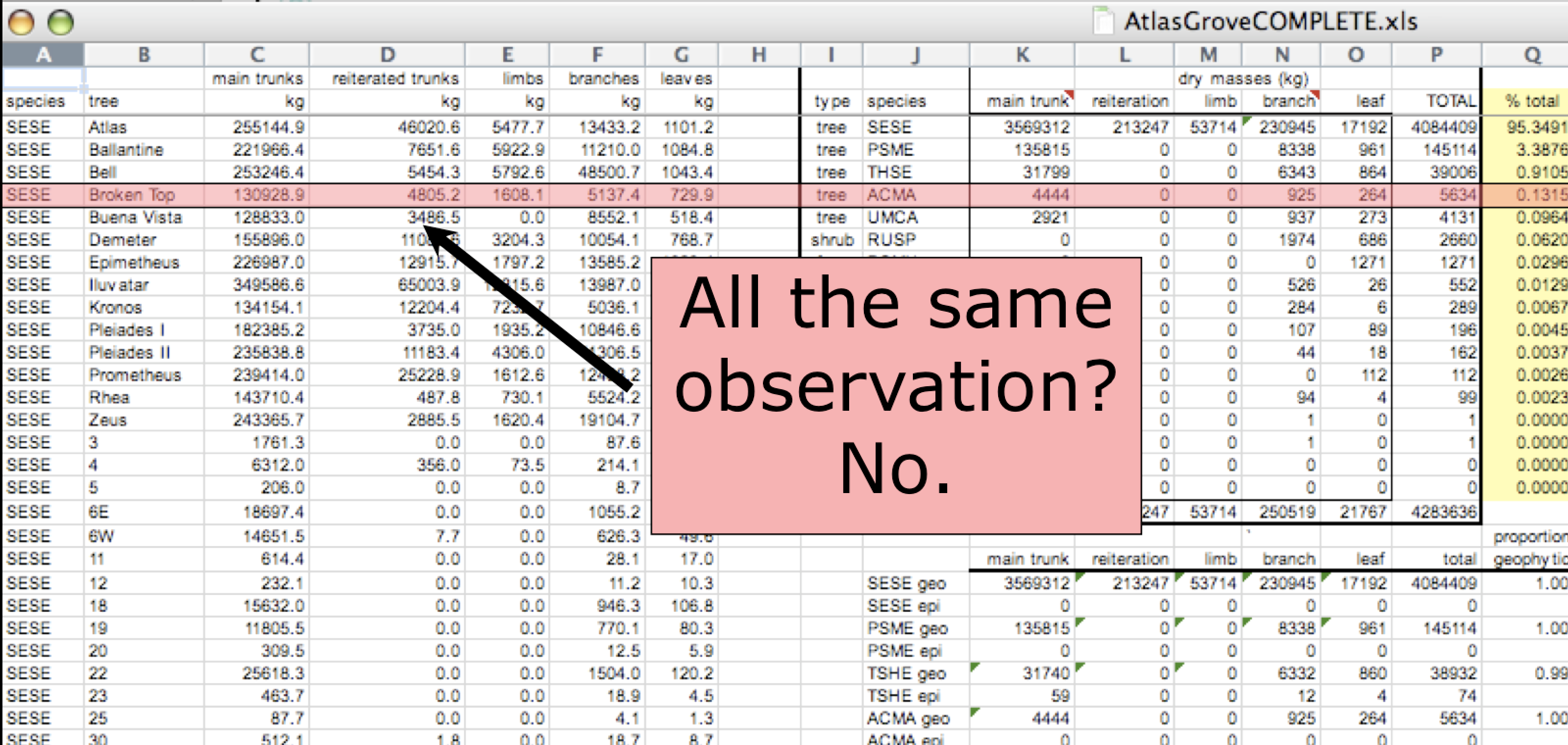
The following is a screenshot of an actual dataset that came across NCEAS. We have all seen spreadsheets that look like this - and it is fairly obvious that whatever this is, it isn’t very tidy.

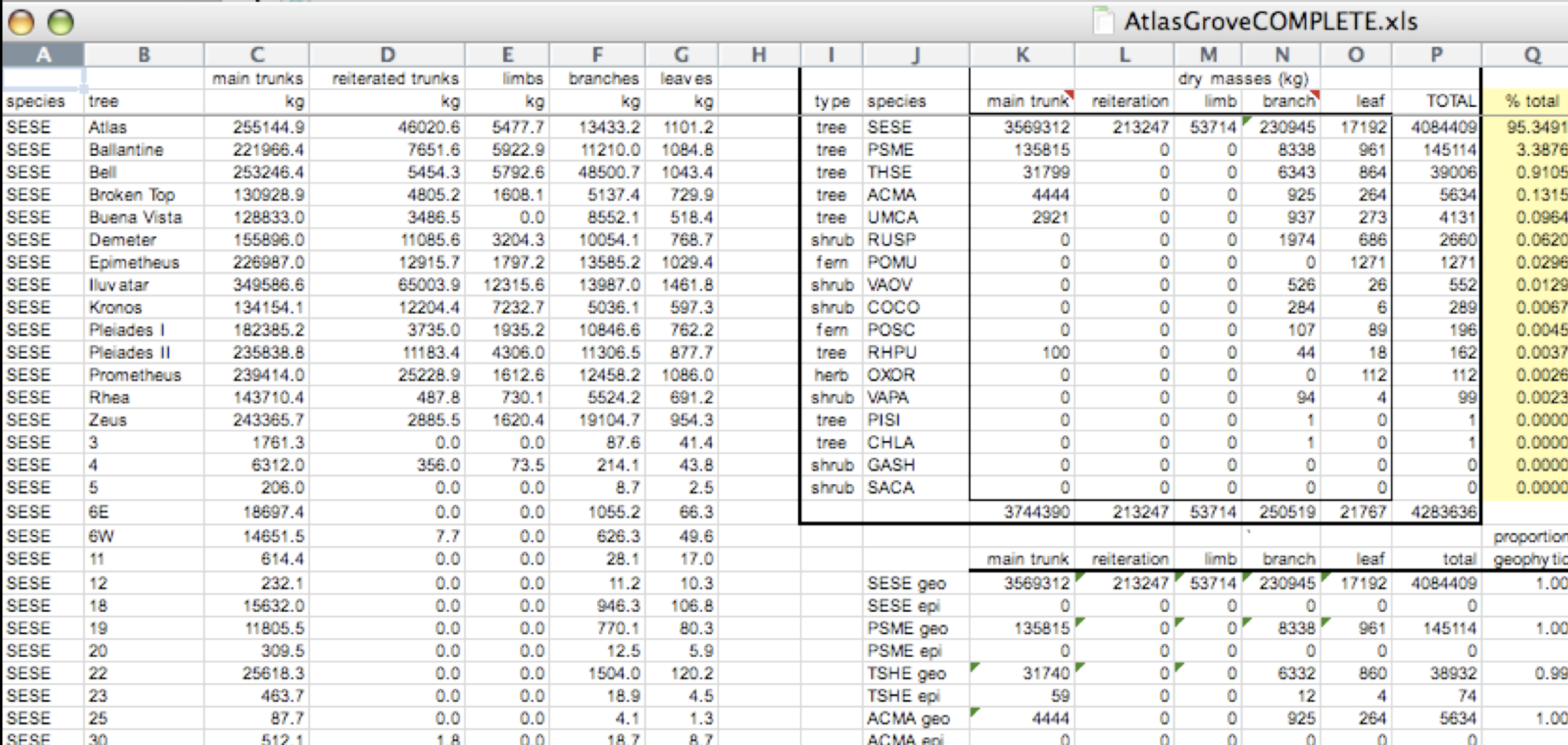
Let’s dive deeper into why we consider this untidy data.

Multiple tables

First, notice there are actually three smaller tables within this table. Although for our human brain it is easy to see and interpret this, it is extremely difficult to get a computer to see it this way. Having multiple tables immediately breaks the tidy data principles, as we will see next.

Inconsistent columns (variables)

In tidy data, each column corresponds to a single variable. If you look down a column, and see that multiple variables exist in the table, the data are not tidy. A good test for this can be to see if you think the column consists of only one unit type.

Inconsistent rows (observations)

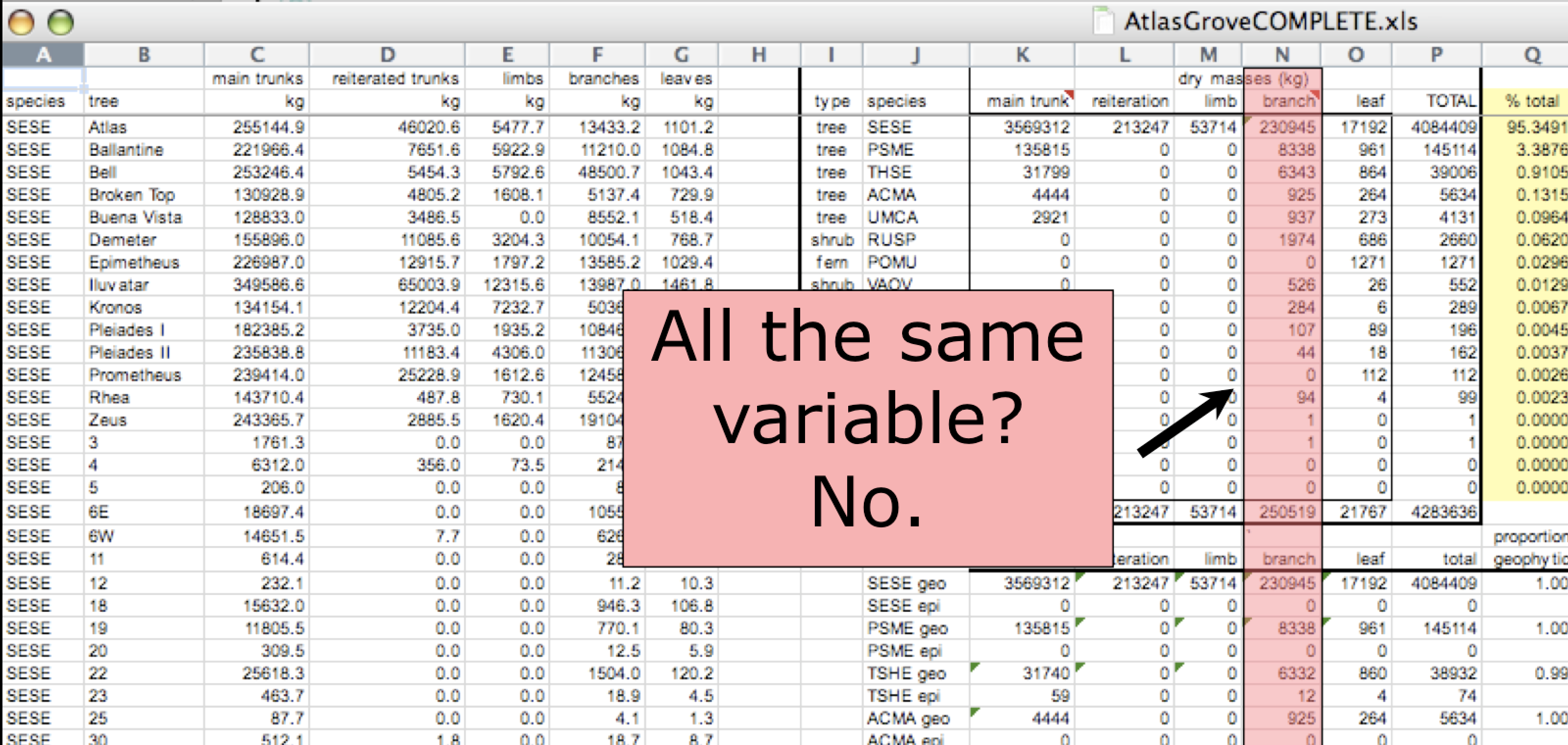
In tidy data, each row must be a single observation. If you look across a single row, and you notice that there are clearly multiple observations in one row, the data are likely not tidy.

Marginal sums and statistics

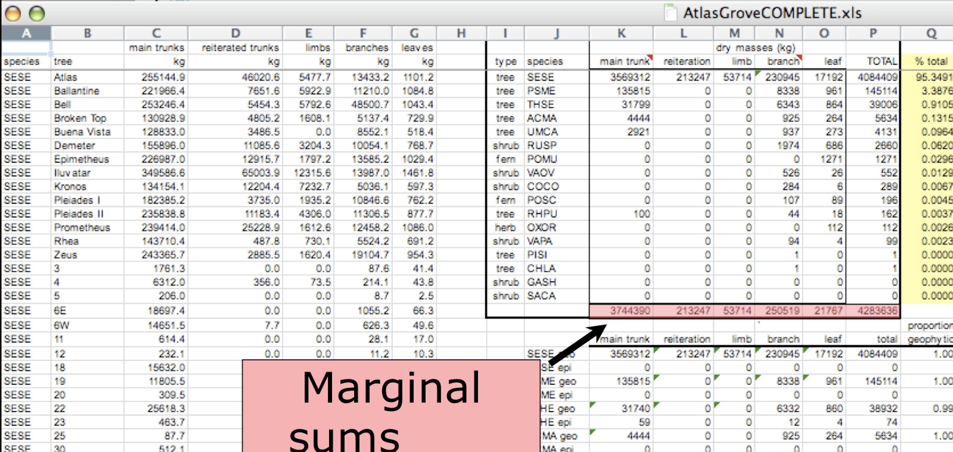
Marginal sums and statistics are not considered tidy. They break the first principle (“Every column is a variable”), because a marginal statistic does not represent the same variable as the values it is summarizing. They also break the second principle (“Every row is an observation”), because they represent a combination of observations, rather than a single one.

6.3 Introduction to the relational data model

The Relational Model, first developed in the late 1960s, provides a highly structured approach for modeling data, and remains the basis for modern relational databases like SQLite, MariaDB, PostgreSQL, and Microsoft Access. It is fully consistent with the tidy data principles, but goes further by providing a formalized framework for decomposing data into multiple tables, while maintaining the relationships between those tables in a way that allows them to be flexibly joined back together on demand.

A database organized following a relational data model is a relational database. However, you don’t have to be using a relational database to enjoy the benefits of using a relational data model, and your data don’t have to be large or complex for you to benefit. Here are a few of the benefits of using a relational data model:

• Enabling powerful search and filtering
• Ability to handle large, complex data sets
• Enforcing data integrity
• Decreasing errors from redundant updates

In this module, we’ll introduce two concepts integral to the relational model. The first involves normalization, and the difference between denormalized and normalized data. The second involves relationships between tables, and different ways of combining records across tables using operations called joins.

6.3.1 Data Normalization

Data normalization is the process of creating normalized data, which are datasets free from data redundancy to simplify query, analysis, storing, and maintenance. In normalized data we organize data so that:

• We have separate tables for each type of entity measured
• Each table follows the tidy data principles
• Each column represents either an identifying variable or a measured variable
• We are not repeating information across rows

In contrast, a denormalized table combines observations about different entities in the same table. A good indication that a data table is denormalized and needs normalization is seeing the same column values repeated across multiple rows. This can sometimes be a convenient way to represent data for certain analysis or visualization tasks, but it is typically an inefficient and error-prone way to manage and store data.

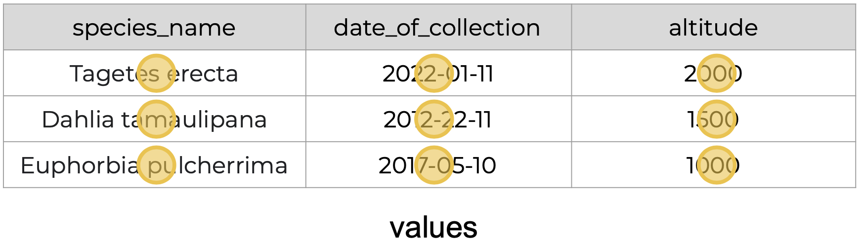
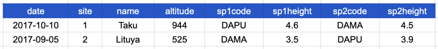
Consider the following table, which shows data about species observed at a specific site and date. The column headers refer to the following:

• date: date when a species was observed
• site: site where a species was observed
• name: site’s name
• altitude: site’s altitude
• sp1code, sp2code: species code for two plants observed
• sp1height, sp2height: corresponding height of the plants observed

Take a moment to see why this is not tidy data.

Challenge

Before reading on, try to answer the following questions:

1. What are the observed entities in the example above?
2. What are the measured variables associated with those observations?

Answer

1. The table has two entities: Site and plants
2. For plant observations, the table records the species names, plant heights, and dates of observation. For sites, the table records the name and altitude.

The table above is not in a normalized form (nor is it tidy!). Each row has measurements about both the site at which observations occurred, as well as observations of two individual plants of possibly different species found at that site.

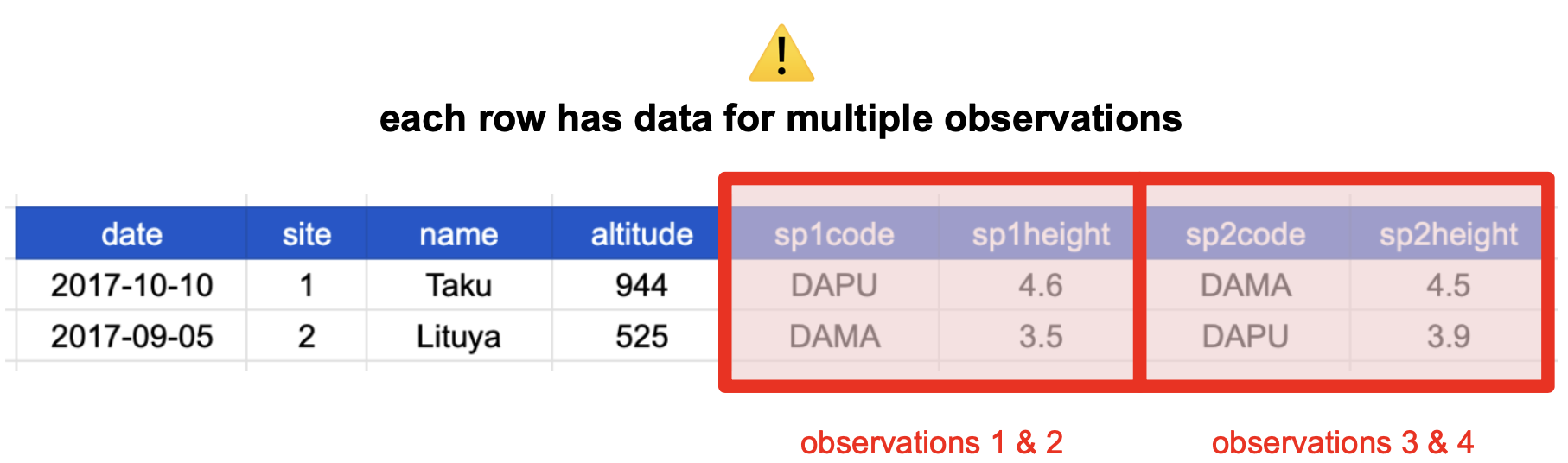
You’ll often see this described as a wide table, because the observations are spread across a wide number of columns. Note that if we observed a new species in the survey, we would need to add new columns to the table. This is difficult to analyze, understand, and maintain.

To solve this problem, we can create a single column for species code, and a single column for species height. The table is now in a long format, which looks like this:

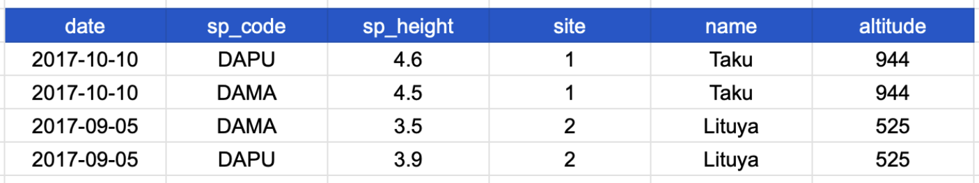
This was an important first step toward normalizing the data, and technically this is now a tidy table. But we’re not done! Notice that in our new table, the row values for the last three columns are repeated.

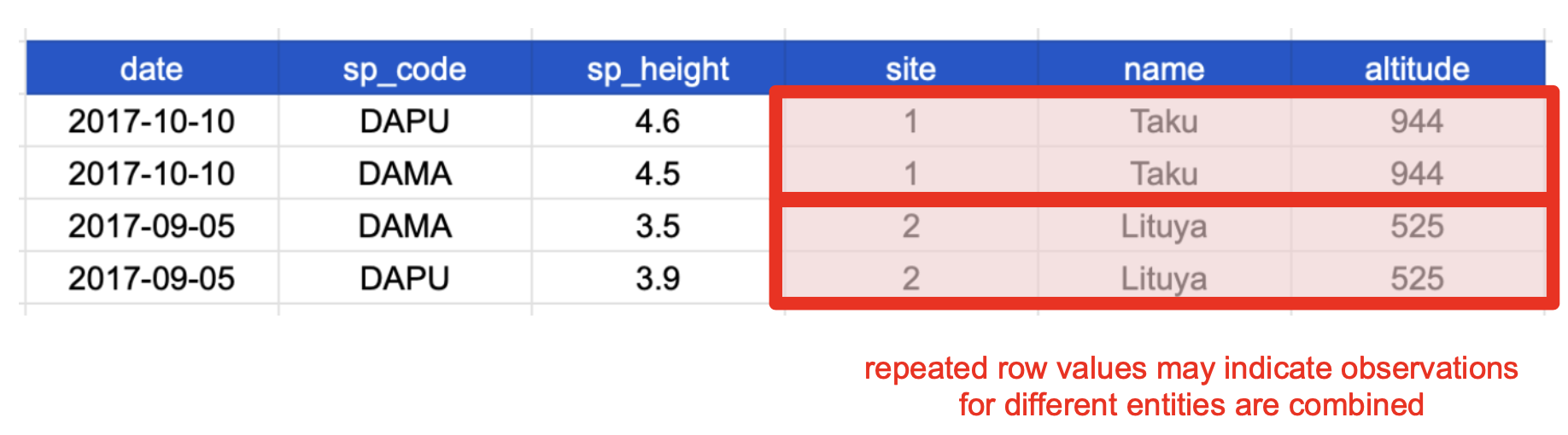
This happens because each row has variables (columns) and values about more than one entity:

• 1st entity: individual plants found at that site
• 2nd entity: sites at which the plants were observed

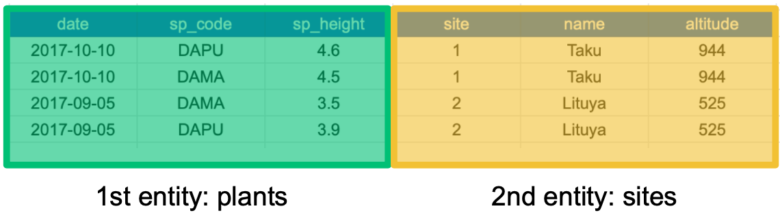
If we use this information to normalize our data, we should end up with:

• one tidy table for plants
• one tidy table for sites
• new columns for uniquely identifying observations (such as site ID)

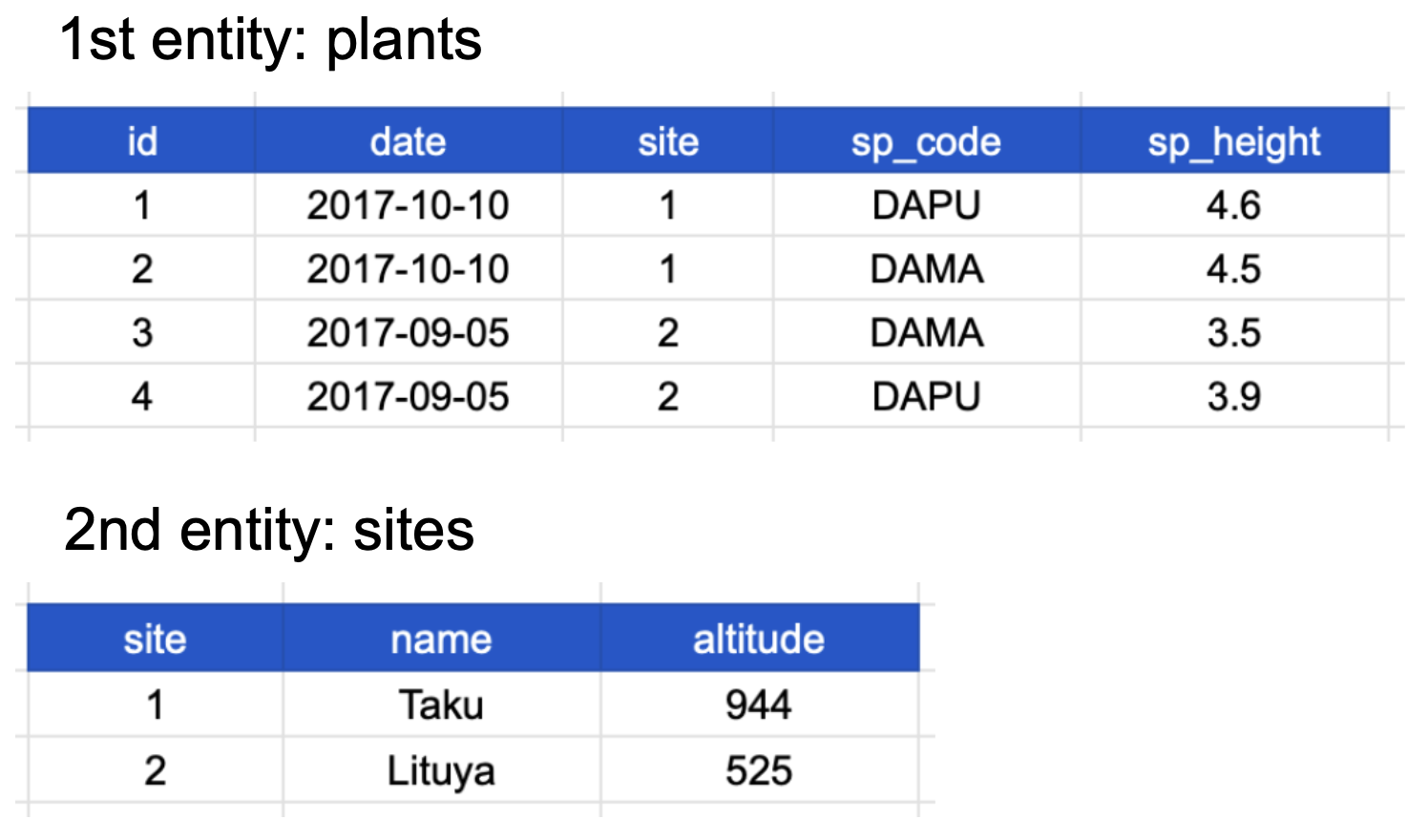
Here’s how our normalized data looks:

Now all of the following are true:

• Separate tables for each type of entity measured
• Each row represents a single observed entity
• Each column represents either an identifier, measured variable, or other attribute of that entity
• All values in a row describe the corresponding observed entity
• All values in a column are of the same type
• Information is not repeated across rows

In addition, notice that each table also satisfies the tidy data principles!

And last but not least, notice that this normalized version of the data meets the three guidelines set by (Borer et al. 2009):

• Design tables to add rows, not columns
• Each column should contain only one type of information
• Record a single piece of data only once; separate information collected at different scales into different tables.

From one table to multiple tables

Normalizing data by separating it into multiple tables often makes researchers really uncomfortable. This is understandable! The person who designed this study collected all of these measurements for a reason - so that they could analyze the measurements together. Now that our site and plant information are in separate tables, how would we use site altitude as a predictor variable for species composition, for example?

We will go over a solution in the next section.

6.3.2 Managing table relationships

To reiterate, the relational data model is not just about decomposing your data into tidy tables, but also connecting those tables to one another so that observations of related entities can linked back together as needed.

This linkage is accomplished via keys, the cornerstone of relational data models. Keys are columns (or combinations of columns) whose values unambiguously identify observations of an entity.

Two types of keys are common within relational data models:

• Primary Key: chosen key for a table, uniquely identifying each observation in the table
• Foreign Key: reference to a primary key in another table, used to create links between tables

Challenge

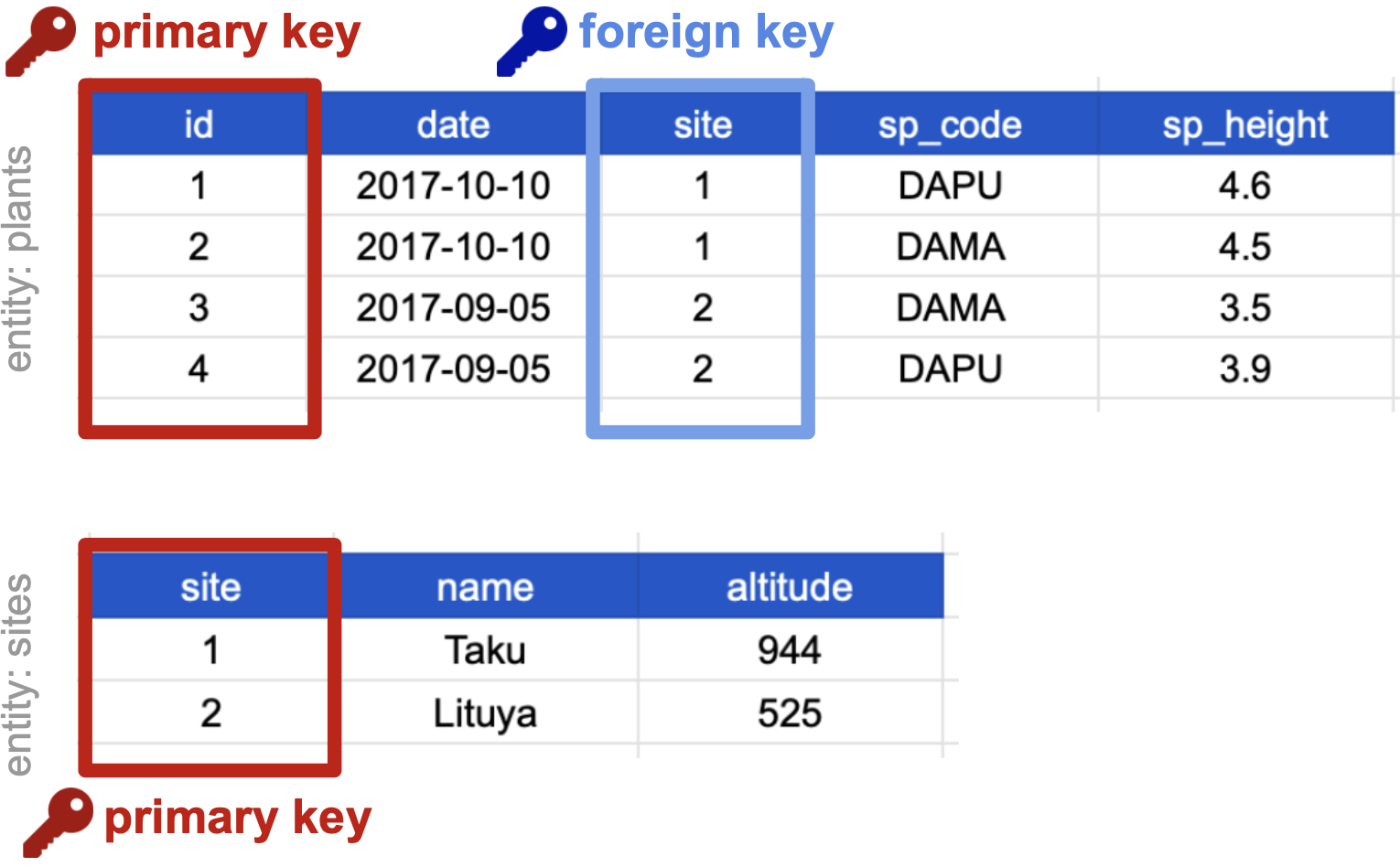
In our normalized tables below, identify the following:

• the primary key for each table
• any foreign keys that exist

Answer

The primary key of the top table is id. The primary key of the bottom table is site.

The site column is the primary key of that table because it uniquely identifies each row of the table as a unique observation of a site. In the first table, however, the site column is a foreign key that references the primary key from the second table. This linkage tells us that the first height measurement for the DAPU observation occurred at the site with the name Taku.

In the examples above, each key corresponds to an individual column in a table. However, it’s also possible to define a key based on multiple columns. Imagine a table containing one unique observation for each date from each site. In that case, although neither date nor site alone uniquely identifies each table record, the combination of these two columns contains all the information we need. Keys made up of two or more columns in a table are called composite keys, and you’ll see a lot of these in practice.

Finally, note that there are various strategies for choosing and/or creating keys when desiging a data model, including natural keys, surrogate keys, and compound keys. Each type of key has advantages and disadvantages. We won’t discuss them more here, but you can read more about it in this article.

6.3.3 Joining tables

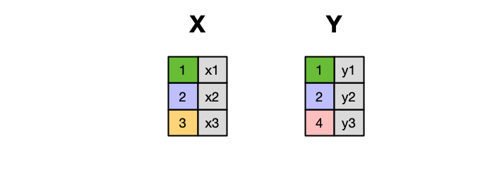
Frequently, analysis of data will require merging these separately managed tables back together. There are multiple ways to join the observations in two tables, based on how the rows of one table are merged with the rows of the other. Regardless of the join we will perform, we need to start by identifying the primary key in each table and how these appear as foreign keys in other tables.

When conceptualizing merges, one can think of two tables, one on the left and one on the right.

6.3.3.1 Inner Join

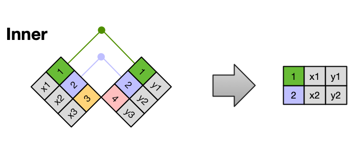
The most common (and often useful) join is when you merge the subset of rows that have matches in both the left table and the right table: this is called an INNER JOIN.

6.3.3.2 Left Join

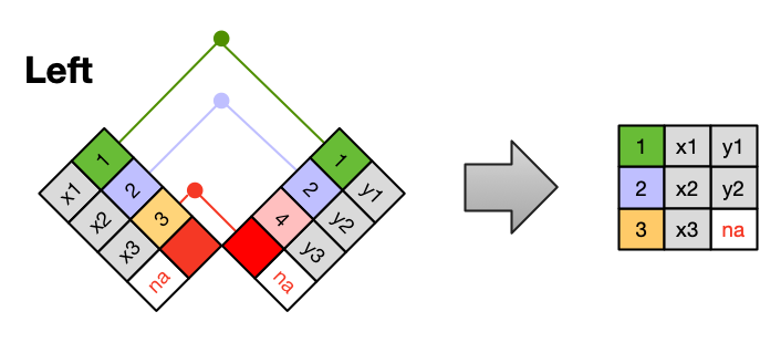
A LEFT JOIN takes all of the rows from the left table, and merges on the data from matching rows in the right table. Keys that don’t match from the left table are still provided with a missing value (na) from the right table.

6.3.3.3 Right Join

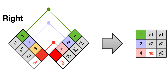
A RIGHT JOIN is the same as a left join, except that all of the rows from the right table are included with matching data from the left, or a missing value. Notice that left and right joins can ultimately be the same depending on the positions of the tables.

6.3.3.4 Full Outer Join

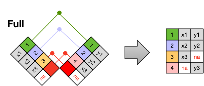
Finally, a FULL OUTER JOIN includes all data from all rows in both tables, and includes missing values wherever necessary.

Sometimes people represent these as Venn diagrams showing which parts of the left and right tables are included in the results for each join. This representation is useful, but it misses part of the story related to where the missing value comes from in each result.

Image source: R for Data Science, Wickham & Grolemund.

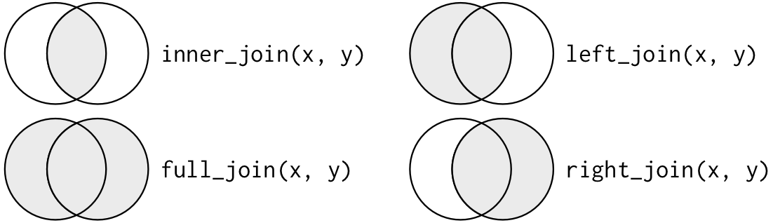
We suggest reading the Relational Data chapter in the “R for Data Science” book for more examples and best practices about joins.

6.3.4 Entity Relationship Diagrams

Entity-relationship modeling is the important process of stepping back to think about your data, deciding what are your entities, their attributes, and the relationships between them. Ideally you will do this early in the process of gather and recording data, but often you’ll need to do it as part of the process of organizing and cleaning up an existing dataset. In either case, an Entity Relationship Diagram (ERD) is a simple but powerful way to compactly describe the structure and relationships of tables in a relational database, including the primary and foreign keys. If you can draw an ERD for your data, it will make it easier to reason about the assumptions you’re making about your data, and validate that your data model is a solid representation of the real-world entities and phenomena captured in your data.

Here are the steps to building up an ERD:

Step 1: Identify your entities

Identify the entities in the relational database and draw a box for each one. In our case, the entities are plants and sites, since we are gathering observations about both of these.

erDiagram
    Plants { }
    Sites { }

Step 2: Add variables and identify keys

In each box, add the variables as a list, identifying all primary keys (PKs) and foreign keys (FKs).

erDiagram
    Plants {
        numeric id PK
        date date
        numeric site FK
        string sp_code
        numeric sp_height
    }
    Sites {
        numeric site PK
        string name
        numeric altitude
    }

Step 3: Add entity relationships and indicate cardinality

First draw a line between each pair of boxes that have a PK-FK relationship, and annotate it to describe how they are related. The “direction” of the relationship is from the table with the FK to the table with the FK. In this example, site is the primary key of Sites and appears as a foreign key in Plants, so we might label Plants as observed_in Sites.

Then quantify how many items in one entity can be related to each observation in another entity. The options are zero, one, many, or some combination thereof. In this case, if every site has one or more plant, we add the symbol for “One or Many” at the end of the line going from Sites to Plants. In the other direction, a plant must be observed in exactly one site, so we add the symbol for “One and ONLY One” at the end of the line going from Plants to Sites.

erDiagram
    Plants |{--|| Sites : observed_in
    Plants {
        numeric id PK
        date date
        numeric site FK
        string sp_code
        numeric sp_height
    }
    Sites {
        numeric site PK
        string name
        numeric altitude
    }

Here is an example of a more complicated ERD, with details about how to indicate the other types of relationships.

Note

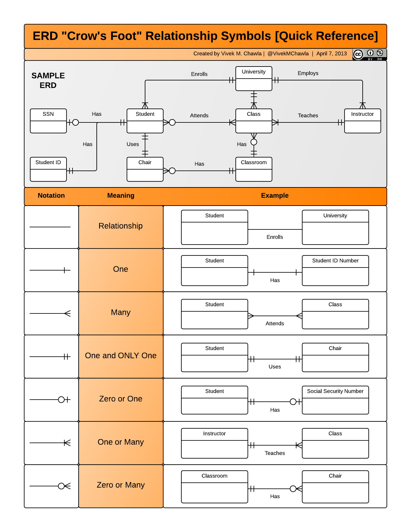
If you need to produce a publishable ERD such as the one above, Mermaid is a great option. Here is the Mermaid “code” used to produce the ERD above for our simple Plants and Sites database. Just like with R code, we can put this in a Quarto code chunk, and it will be used to generate a visual diagram when we render the document.

erDiagram
    Plants |{--|| Sites : observed_in
    Sites {
        numeric site PK
        string name
        numeric altitude
    }
    Plants {
        numeric id PK
        date date
        numeric site FK
        string sp_code
        numeric sp_height
    }

erDiagram
    Plants |{--|| Sites : observed_in
    Sites {
        numeric site PK
        string name
        numeric altitude
    }
    Plants {
        numeric id PK
        date date
        numeric site FK
        string sp_code
        numeric sp_height
    }

Read more here about how to use this tool to create diagrams.

6.4 Data modeling exercise

Let’s practice what we’ve learned!

In this exercise, we’ll be working with a tidied up version of a dataset from ADF&G containing commercial catch data from 1878-1997. The dataset and reference to the original source can be viewed at its public archive: https://knb.ecoinformatics.org/#view/df35b.304.2. That site includes metadata describing the full data set, including column definitions.

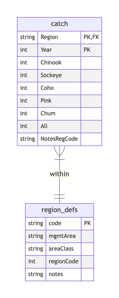
Here’s the first catch table:

And here’s the region_defs table:

Challenge

Using the live session started by your instructor, work through the following tasks:

Part 1. Draw an Entity Relationship diagram for the tables, including labels as relevant for primary and foreign keys, along with entity relationships and corresponding cardinality.

Part 2. Is the catch table in normal (aka tidy) form? If so, what single type of entity was observed? If not, how might you restructure the data to make it normalized, tidy, and well-modeled overall? Draw a new ERD for your new tables, again detailing all keys and relationships.

Solution

Part 1. We can start by creating one box for each of the two tables in the dataset. We have a catch table with annual catch by region for several species, and region_defs table with one record for each region. Next, we list all of the columns contained within each table.

What about keys? The catch table does not have a column uniquely identifying each record! However, given that the observations here are catch within region by year, the combination of region and year does the trick. To denote this composite primary key, we can label both fields as PK in this table.

Meanwhile, the region table appears to use code to uniquely identify each region, and this field is referenced in the catch table. So we’ll label code as the PK within the region_defs table, and label the corresponding (but differently named!) Region field as FK in the catch table. Note that the region_defs table also somewhat confusingly has a regionCode field, which superficially sounds like a candidate primary key. However, looking at the data, it is clearly that this does not uniquely identify each record in the region_defs table, nor is it referenced from the catch table.

Finally, let’s document the relationships. Each annual catch record counts fish caught within a particular region, so we definitely need a line between them to express this relationship. What is the cardinality? Clearly each catch record belongs to exactly one region, so we’ll use “one and ONLY one” on the region_defs side. Meanwhile, there can be many catch record per region. We could simple choose to label this as “many” cardinality, but let’s be more specific and label it as “one or many”; this asserts that the region table only contain regions that have at least one catch record.

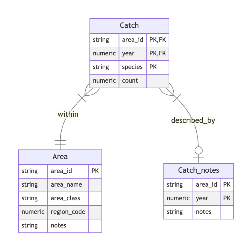
Part 2. There are number of changes we might make here! There’s no single correct answer, but here are some improvements you might consider.

• The catch table is clearly not tidy, using a wide format. Let’s first pivot that to a long format, retaining the existing region and year identifier fields, then adding a single species field with a corresponding count (of fish caught) field.
• As part of the previous step, note that we’ve eliminated the All field. If this is the sum of the species counts, then it a marginal statistic, and not considered tidy. We could always recompute it later by summing over all of the species-specific counts. If this is not (always) the sum of individual counts, then this raises questions about where the values come from, and could lead us to consider bigger changes in how the data is recorded and how the tables is designed. For this exercise, let’s just assume its a marginal sum, and discard the column.
• While we’re at it, let’s address the confusion around multiple meanings for “region”, and corresponding inconsistency in table and field names. According to the documention, the catch counts are really by area, and areas are located within regions identified by the regionCode field. So let’s rename our region_defs table to Area, and make its field names more consistent by renaming code to area_id, mgmtArea to area_name, and areaClass to area_class.
• For consistency with common (although by no means required) convention, let’s also use lower case in all field names, while capitalizing table names.
• Finally, let’s consider the NotesRegCode. Strictly speaking, in the original tables, each value corresponds to the observed catch for a given year and region. If we kept this field in our new Catch table in long format, it would be repeated for each species observation in a given year and area, and therefore would not be tidy. To retain the original semantics, we can put these notes in a new table called Catch_notes, with a composite primary key based on area_id and year. Those two matching columns in the Catch table would therefore be FKs to the Catch_nodes table, and we might say that that catch observations are described_by catch notes. With respect to cardinality, we see in the data that not all observations have an associated note, while it’s clear that with our new long Catch table, any given note will refer to all species-level observations within each area and year. Hence let’s indicate that catch observations are described by “zero or one” notes, and notes describe “one or many” species catch observations.

Here’s an ERD reflecting the changes describe above.

Bonus challenge

If you have time, take on this extra challenge with your group.

Navigate to this dataset: Richard Lanctot and Sarah Saalfeld. 2019. Utqiaġvik shorebird breeding ecology study, Utqiaġvik, Alaska, 2003-2018. Arctic Data Center. doi:10.18739/A23R0PT35

Read the dataset documention, inspect the tables, and then try to create an ERD that includes the following tables from the package:

• Utqiagvik_adult_shorebird_banding.csv
• Utqiagvik_egg_measurements.csv
• Utqiagvik_nest_data.csv
• Utqiagvik_shorebird_resightings.csv

6.5 Resources

• Borer et al. 2009. Some Simple Guidelines for Effective Data Management. Bulletin of the Ecological Society of America.
• White et al. 2013. Nine simple ways to make it easier to (re)use your data. Ideas in Ecology and Evolution 6.
• Software Carpentry SQL tutorial
• Tidy Data

Borer, Elizabeth, Eric Seabloom, Matthew B. Jones, and Mark Schildhauer. 2009. “Some Simple Guidelines for Effective Data Management.” Bulletin of the Ecological Society of America 90: 205–14. https://doi.org/10.1890/0012-9623-90.2.205.