Learning Objectives
- Explain the importance of using and developing functions
- Create custom functions using R code
- Document functions to improve understanding and code communication
12.1 Function fundamentals
Many people write R code as a single, continuous stream of commands, often drawn from the R console itself and simply pasted into a script. While any script is preferable to non-scripted solutions, there are advantages to breaking code into small, reusable modules. This is the role of a function in R. In this lesson, we will review the advantages of coding with functions, practice by creating some functions and show how to call them, and then do some exercises to build other simple functions.
In general, a function is a defined set of code statements or expressions that are organized together to perform a specific task, and can be used (aka “called”) whenever needed. Functions are typically designed to accept some input(s), do something with it, and return a useful output. Sometimes a function may be designed to have one or more side effects, such as printing something to the console or saving a file to disk, but today we will focus only on functions that simply return a result. Functions are common in all major programming languages, including R.
There are many advantages to writing small functions that only complete one logical task and do it well:
- When you need to modify your code, you only need to update it in one place.
- You can make the code easier to understand by giving an informative name to your function.
- You can take advantage of iteration techniques that apply a function to each member of a collection. For example,
dplyr::acrossallows you to apply the same function to multiple columns of a data frame all in one expression.
Functions are essential for following the DRY principle in coding and softward development: Don’t Repeat Yourself!
12.2 Functions in R
In R, functions are objects that can be created and assigned to a name so that they can be used throughout code by reference – just like vectors, data frames, and other types of objects! To create a function in R, you use the function function (so meta!). Here is the general template for a function definition:
<function_name> <- function(<argument1>, <argument2>, ...) {
  <whatever code your function needs to run>
  return(<something>)
}
The function arguments, specified in parentheses after the function keyword and separated by commas, are placeholders for the inputs that we want our function to accept. A function might have just one argument, or many arguments, or even zero arguments if the function does not require any inputs when called! After listing the arguments, we provide the function body enclosed in squiggly braces ({}). This is the code that will be run everytime the function is called. Typically your code will operate on (or otherwise use) the provided arguments. Note that the final line of the function body is a return(<something>) expression, where <something> is a single object - e.g. a vector, a list, a data frame, or even another function! Technically, if you don’t include a return(), R will simply return the result of the last expression it evaluates in the function body. However, it’s good practice to use an explicit return in most cases. Finally, notice that we assign the entire function definition, i.e. function(...) {...}, to a name. Just like when creating vector and data frames, we need to assign a function to a name in order to be able to refer to it again later.
Note that if your function body refers to named objects that you have neither passed in as arguments nor created inside your function body, R will apply so-called scoping rules that dictate where it will look outside the function for that named object. Scoping rules are, ahem, outside the scope of this module. But as a general rule, to avoid complexity and bugs, your function body should only operate on variables that you have passed in as objects.
12.3 Exercise: Temperature Conversion
Imagine you have some multiple sets of temperature readings in units of Fahrenheit, and need to convert it to Celsius. You might write an R script that does this for you.
interior_f <- c(175, 134, 181)
interior_c <- (interior_f - 32) * 5/9

exterior_f <- c(77, 78, 77)
exterior_c <- (exterior_f - 32) * 5/9

surface_f <- c(103, 102, 99)
surface_c <- (surface_f - 32) * 5/9
Note the duplicated code, which repeats the same formula three times. What if you realized your formula had an error? You would need to correct it in three places. Moreover, it would be hard to notice if one of the conversion statements contained a typo in the formula. Overall, the code would be more compact and more reliable if we didn’t repeat ourselves.
Write a temperature conversion function
Let’s create a function that calculates Celsius temperature outputs from Fahrenheit temperature inputs.
convert_f_to_c <- function(fahr) {
  celsius <- (fahr - 32) * 5/9
  return(celsius)
}
By running this code, we have created a function object and stored it in the R global environment. The fahr argument to the function function indicates that our conversion function expects a single argument (the temperature in Fahrenheit), and the return statement indicates that the function should return the value in the celsius variable that was calculated inside the function. Let’s use it, and check if we got the same value as before:
surface_c_v2 <- convert_f_to_c(fahr = surface_f)
surface_c_v2
[1] 39.44444 38.88889 37.22222identical(surface_c_v2, surface_c)[1] TRUEExcellent! Now we have our own local function for converting a vector of temperatures in Fahrenheit to temperatures in Celsius. Note also that we explicitly named the argument inside the function call (convert_f_to_c(fahr = surface_f)), but in this simple case, R can figure it out if we didn’t explicitly tell it the argument name (convert_f_to_c(surface_f)). More on this later!
Your Turn: Create a Function that Converts Celsius to Fahrenheit
Create a function named convert_c_to_f that does the reverse, taking temperatures in Celsius as input and returning them in Fahrenheit.
Create the function convert_c_to_f in a new code chunk or even a separate R script file.
Then use that formula to convert the Celsius vectors back into Fahrenheit values, and compare the results to the original Fahrenheit vectorto ensure that your answers are correct.
Hint: the formula for Celsius to Fahrenheit conversions is celsius * 9/5 + 32.
Did you encounter any issues with rounding or precision?
12.4 Exercise: Minimizing Work with Functions
Functions can be as simple or complex as needed. They can be very effective in repeatedly performing calculations, or for bundling a group of commands that are used on many different input data sources. For example, we might create a simple function that takes Fahrenheit temperatures as input, and calculates both Celsius and Kelvin temperatures. All three values are then returned in a list, making it very easy to create a comparison table among the three scales.
convert_temps <- function(fahr) {
  celsius <- (fahr - 32) * 5/9
  kelvin <- celsius + 273.15
  return(list(fahr = fahr, celsius = celsius, kelvin = kelvin))
}

surface_temps_df <- data.frame(convert_temps(fahr = surface_f))
But what if we wanted to make this function more flexible? For example, what if wanted to allow the user to provide temperatures in either Fahrenheit or Celsius? Let’s add an additional argument so the user can specify the input units. While we’re at it, let’s also add some error checking, and update the function to return the result as a data frame rather than a list.
convert_temps2 <- function(temp, unit = "F") {

  ### Error checking:
  unit <- toupper(unit)  ## try to anticipate common mistakes!
  if (!unit %in% c("F", "C")) {
    stop("The units must be either F or C!")
  }

  if (unit == "F") {
    fahr <- temp
    celsius <- (fahr - 32) * 5/9
  } else {
    celsius <- temp
    fahr <- celsius * 9 / 5 + 32
  }
  kelvin <- celsius + 273.15

  out_df <- data.frame(fahr, celsius, kelvin)
  return(out_df)
}

# run on the Celsius values, using named arguments
surface_temps_df1 <- convert_temps2(temp = surface_c, unit = "C")

# run on the Fahrenheit values, using positional arguments
surface_temps_df2 <- convert_temps2(surface_f, "F")

# run on the Fahrenheit values, using default `unit` of "F"
surface_temps_df3 <- convert_temps2(surface_f)

# check that the last output matches our earlier data frame
identical(surface_temps_df, surface_temps_df3)
[1] TRUENotice that we added some other new features here as well. In the arguments list of our function definition, we provided a default value for the unit argument (unit = "F"). This convenience means that the function caller can opt to skip that argument, and R will use the default value. Because temp does not have a default, the user cannot skip that one! Also note that R interprets the arguments in order, so we can even skip naming them, though when calling novel or complex functions it is helpful to explicitly name the arguments.
12.5 Functions in the tidyverse
If you frequently work with the tidyverse package and all its amazing functionality, understanding how those tidyverse functions are designed can help you write your own tidyverse style functions. There are two common use cases:
- A function that can be used to calculate inside a
mutate()orsummarize() - A function that can be used seamlessly in a piped
tidyverse-style workflow
12.5.0.1 Functions for mutate or summarize
This kind of function should take a vector (or multiple vectors) and return a single vector. Functions that return a vector the same length as the input would be useful for mutate(); functions that return a vector of length 1 (e.g., mean() or sd()) would be useful for summarize(). We’ve already created two functions like that.
data.frame(f = surface_f) %>%
  mutate(c = convert_f_to_c(fahr = f),
         f2 = convert_c_to_f(celsius = c))
f c f2
1 103 39.44444 103
2 102 38.88889 102
3 99 37.22222 99Why wouldn’t our convert_temps() function work here?
12.5.0.2 Functions for piped workflows
A common workflow in the tidyverse is to use the magrittr pipe operator %>% (or the newer built-in |>) to pass a data frame into a function like select(), filter(), or mutate(), and then pass the results from that into another function, and so on:
surface_temps_df %>%
  select(fahr, celsius) %>%
  mutate(rankine = fahr + 459.67)
fahr celsius rankine
1 103 39.44444 562.67
2 102 38.88889 561.67
3 99 37.22222 558.67For this to work:
- Every
dplyrandtidyrfunction takes a data frame (or variant such as a tibble) as its first argument. - Every
dplyrandtidyrfunction returns a data frame (or variant).
The pipe operator %>% says, take the preceding object (a data frame, such as one returned by a dplyr function) and pass it to the next function (such as another dplyr function) as the first argument.
12.6 Exercise: Make a tidyverse style function
Let’s make a function that can take a dataframe and calculate a new column that tells whether a temperature is hot or cold, based on some threshold.
add_hot_or_cold <- function(df, thresh = 70) {
  ### error check:
  if (!"fahr" %in% names(df)) {
    stop('The data frame must have a column called `fahr`!')
  }

  out_df <- df %>%
    mutate(hotcold = ifelse(fahr > thresh, "hot", "cold"))

  return(out_df)
}

surface_temps_df %>%
  select(fahr, celsius) %>%
  add_hot_or_cold(thresh = 100) %>%
  arrange(desc(fahr))
fahr celsius hotcold
1 103 39.44444 hot
2 102 38.88889 hot
3 99 37.22222 cold12.7 Functions and ggplot()
Once we have a dataset like that, we might want to plot it. One thing that we do repeatedly is set a consistent set of display elements for creating graphs and plots. By using a function to create a custom ggplot theme, we can enable to keep key parts of the formatting flexible. For example, in the custom_theme function, we provide a base_size argument that defaults to using a font size of 9 points. Because it has a default set, it can safely be omitted. But if it is provided, then that value is used to set the base font size for the plot.
custom_theme <- function(base_size = 9) {
  ### NOTE: functions used *inside* a function need to be available,
  ### e.g., attached with library() or called using namespace (package::function)
  ggplot2::theme(
    text = element_text(family = "serif",
                        color = "gray30",
                        size = base_size),
    plot.title = element_text(size = rel(1.25),
                              hjust = 0.5,
                              face = "bold"),
    panel.background = element_rect(fill = "azure"),
    panel.border = element_blank(),
    panel.grid.minor = element_blank(),
    panel.grid.major = element_line(colour = "grey90",
                                    linewidth = 0.25),
    legend.position = "right",
    legend.key = element_rect(colour = NA,
                              fill = NA),
    axis.ticks = element_blank(),
    axis.line = element_blank()
  )
}

library(ggplot2)

ggplot(surface_temps_df, aes(x = fahr, y = celsius, color = kelvin)) +
  geom_point() +
  custom_theme(10)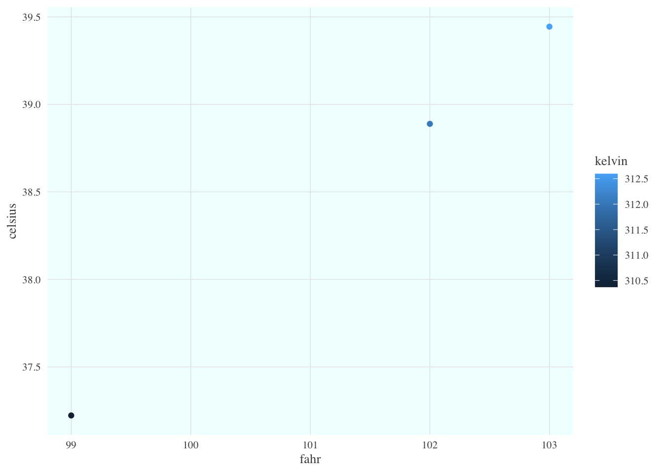
In this case, we set the font size to 10, and plotted the air temperatures. The custom_theme function can be used anywhere that one needs to consistently format a plot.
But we can go further. One can wrap the entire call to ggplot in a function, enabling one to create many plots of the same type with a consistent structure. For example, we can create a scatterplot function that takes a data frame as input, along with a point_size for the points on the plot, and a font_size for the text.
scatterplot <- function(df, point_size = 2, font_size = 9) {
  ggplot(df, mapping = aes(x = fahr, y = celsius, color = kelvin)) +
    geom_point(size = point_size) +
    custom_theme(font_size)
}
Calling that lets us, in a single line of code, create a highly customized plot but maintain flexibility via the arguments passed in to the function. Let’s set the point size to 3 and font to 16 to make the plot more legible.
scatterplot(surface_temps_df, point_size = 3, font_size = 16)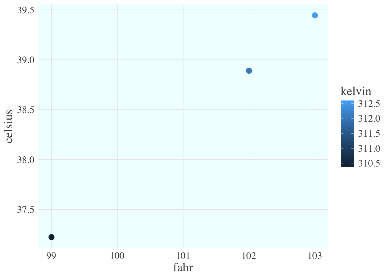
Once these functions are set up, all of the plots built with them can be reformatted by changing the settings in just the functions, whether they were used to create 1, 10, or 100 plots.
12.8 Summary
- Use functions to make code less repetitive, more understandable, and ultimately more robust
- Build functions in R with
function() - Design R functions to work with
tidyverseflow